REVIEW 3 major objections 5 minor 53 references
Practical Application of the Quantum Carleman Lattice Boltzmann Method in Industrial CFD Simulations
T0 review · 3 major / 5 minor · reviewed 2026-08-16 · deepseek-v4-flash
Pith's one-line read The paper claims that an HHL quantum linear solver applied to a Carleman-linearized lattice Boltzmann system solves benchmark two-dimensional flows with median error fidelities near $10^{-3}$, and that small-lattice eigenvalue spectra can…
desk verdict A careful statevector-emulation benchmark of the Carleman-LBM plus HHL pipeline on three toy 2D flows; the 10^-3 fidelity is a circuit check, the Carleman error is ~5%, and the spectral-transfer claim is real but only validated on lattices commensurate with 4. read the letter →
The pith
A machine-rendered reading of the paper's core claim, the machinery that carries it, and where it could break.
The reading
What carries the argument
The load-bearing object is the matrix $A$ that encodes the Carleman-linearized lattice Boltzmann evolution. Carleman linearization introduces auxiliary variables such as $g_{ij}(t,n,m)=f_i(t,n)f_j(t,m)$, turning the nonlinear BGK collision step into a linear update $\varphi(t+dt)=C\varphi(t)$; stacking $N_t$ such updates gives a block-bidiagonal linear system $\tilde A x=b$ whose solution contains the whole time history, and HHL solves the Hermitian form $A$ obtained by placing $\tilde A$ and its adjoint off-diagonal. The spectral-transfer argument is about this matrix: with the number of time steps fixed, the positive eigenvalue density of $A$ is nearly independent of lattice size, so a spectrum obtained once on a 4-by-4 lattice calibrates the controlled rotations of HHL for larger lattices.
What would settle it
Run the same pipeline on a 32-by-32 or larger lattice (or with more than seven time steps), compute the true spectrum of $A$ for that lattice, and compare HHL solutions obtained with the true spectrum against those obtained with the 4-by-4 spectrum; if the bin-wise discrepancy $\zeta$ grows beyond a few percent or the fidelity residual rises above $10^{-4}$, the spectral-transfer shortcut fails. The paper's own $\zeta$ metric and residual plots make this a direct check.
Extended reading notes
Core claim
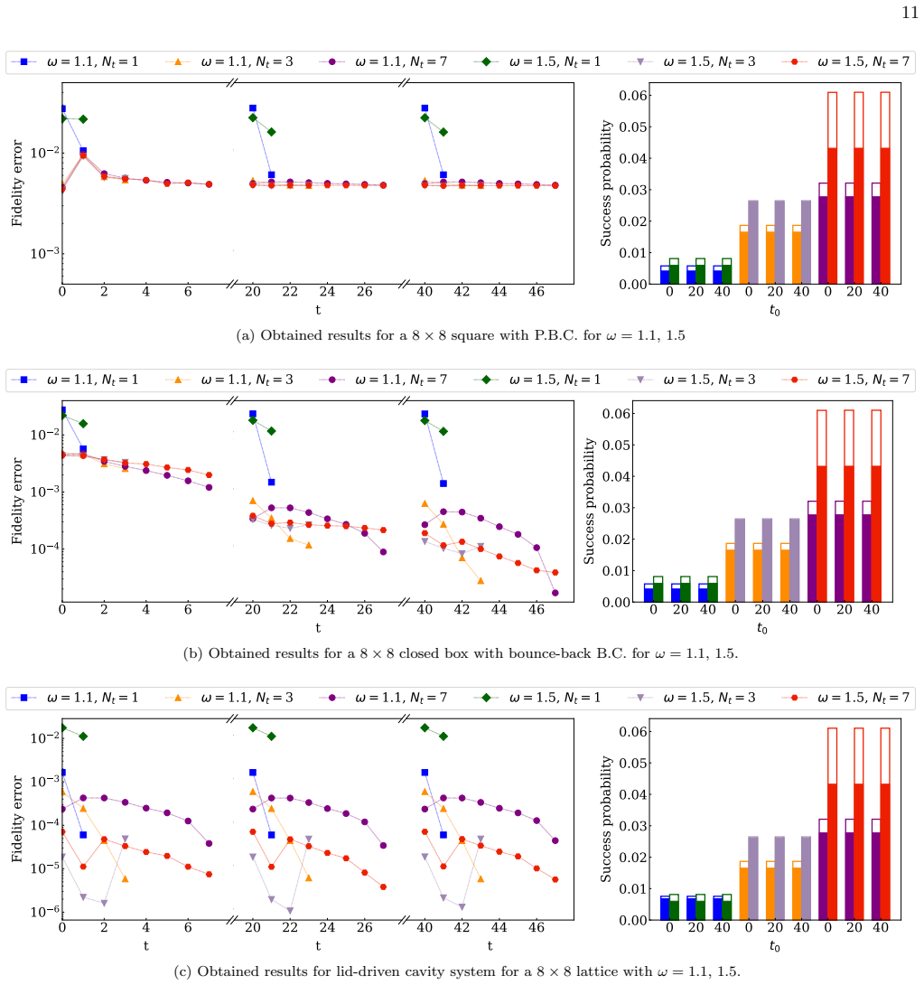
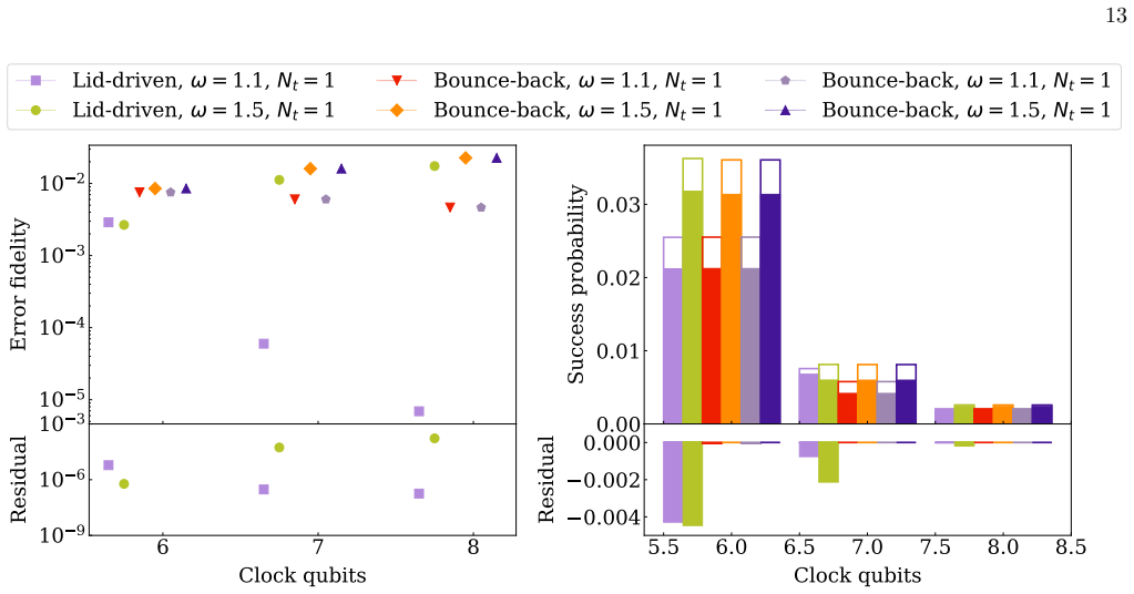
On the paper's own terms, the central discovery is that the Carleman–HHL combination works numerically for all three boundary-condition classes. For single-step evolution the HHL solution matches the exact Carleman solution with fidelity error typically between $10^{-4}$ and $10^{-2}$ depending on clock qubits and relaxation frequency; for multi-step evolution the median error stays near $10^{-3}$ while the success probability grows. The spectral-transfer observation is the second finding: for a fixed number of time steps, the positive part of the spectrum of the matrix $A$ is nearly identical for $N_x = 4,8,12$ after one step, and still within a few percent bin-wise discrepancy after seven steps. Using the 4-by-4 spectrum in place of the true 12-by-12 or 20-by-20 spectrum leaves the fidelity error nearly unchanged, with residuals below $10^{-4}$. This is presented as evidence that eigenvalue pre-evaluation, normally one of HHL's serious bottlenecks, can be amortized over a family of lattice sizes.
Load-bearing premise
The load-bearing premise is that the eigenvalue pattern of a tiny 4-by-4 lattice stays representative of larger lattices; the paper verifies this numerically only up to a 20-by-20 lattice and seven time steps, and it supplies no proof or error bound for the transfer.
Editorial extensions
If this is right
- First-order Carleman truncation is enough for the tested flows: it matches the second-order accuracy in most parameter regimes while costing far less, so the cheaper pipeline can be used in practice.
- Spectral transfer directly attacks one of HHL's bottlenecks: a spectrum computed on a 4-by-4 lattice can be reused for 12-by-12 and 20-by-20 lattices with fidelity residuals below $10^{-4}$.
- Encoding more time steps into a single HHL solve is the right strategy: success probability rises with the number of encoded time steps while fidelity stays near $10^{-3}$, so reusing the same circuit for long times is worse than adding time-qubits.
- The dominant error in the combined method is the Carleman truncation itself (about 5%) rather than the HHL solve (under 3%), so raising the truncation order is the next accuracy lever, and its qubit cost grows only linearly in the Carleman order.
Reading between the lines
- The spectral transfer result suggests a production workflow the authors do not spell out: eigenvalue spectra could be precomputed once per boundary-condition class and Reynolds number, making HHL's eigen-decomposition an amortized pre-processing cost rather than a per-simulation cost.
- The near size-independence of the spectrum is plausibly inherited from the local block structure of the Carleman matrix, in which the same small block is repeated across lattice sites; this points toward a rigorous bound on the discrepancy $\zeta$ in terms of $N_x$ and boundary-condition effects, which the paper does not provide.
- The success probabilities are obtained under exact state-vector emulation; the CNOT-count estimates in the appendix indicate that circuit depth, not the spectral shortcut, is likely to decide practicality on near-term quantum hardware, so the next test should be noise-aware.
Signed reviews
Editorial analysis
A structured set of objections, weighed in public.
Referee Report
Summary. This paper presents a statevector-emulated hybrid quantum-classical pipeline for two-dimensional D2Q9 lattice Boltzmann simulations. The nonlinear collision step is linearized with a first-order Carleman expansion, and the resulting multi-step linear system of the form \tilde{A} x = b (Eqs. 21-27) is solved with HHL, using exact spectra of the linear operator A. The authors benchmark three cases (periodic, bounce-back, and lid-driven cavity), quantify the Carleman truncation error against classical LBM (Sec. V A), and report HHL fidelity and success probability as functions of clock qubits, lattice size, and time steps (Secs. V C-D). They further propose using the eigenspectrum of an Nx=4 lattice for larger Nx, claiming negligible fidelity loss (Sec. V E). The headline results are median error fidelities on the order of 10^-3 and success probabilities described as sufficient for practical quantum state sampling.
Significance. The paper is a useful engineering-oriented numerical study: it separates Carleman linearization error from HHL implementation error, tests several boundary conditions, and provides explicit spectral data. If the spectral-transfer result holds for general lattice sizes, it would be a concrete step toward reducing HHL eigenvalue-estimation cost, a known bottleneck. However, the reported 10^-3 fidelity measures agreement with the exact solution of the linear system HHL is designed to solve, not with the physical LBM flow; the physical-model error is the Carleman RMSE, which reaches about 5% (Figs. 4-5). The spectral-transfer claim is supported only by commensurate lattices and lacks an error bound. The paper is honest about the Carleman error and about using exact statevector emulation, but the abstract's wording overstates the level of validation.
major comments (3)
- [Abstract; Sec. V C, Eq. (34)] The 'error fidelity' in Eq. (34) compares the HHL output with the exact solution of the Carleman linear system A x = b, not with the physical LBM solution. The abstract's claim of 'median error fidelities on the order of 10^-3' is therefore a statement about circuit-level consistency, while the physical accuracy is governed by the Carleman truncation error reported separately in Sec. V A, which reaches about 5% (Figs. 4 and 5). Please state this distinction explicitly in the abstract and conclusions, and avoid presenting the internal fidelity as evidence of physical validity.
- [Sec. V B, Sec. V E, Eq. (33), Figs. 12-13] The spectral-transfer claim is tested only for lattices with Nx divisible by 4 (Nx=8, 12, 20; Secs. V B and V E). For the periodic and bounce-back streaming operators the eigenmodes are labeled by wavenumbers 2\pi m/Nx, so the Nx=4 modes are embedded in the target spectrum only when Nx is a multiple of 4. Non-commensurate sizes such as Nx=6, 10, 14, 18 are never tested, and the zeta metric in Eq. (33) is a binned count of missing bins rather than a per-eigenvalue error weighted by the initial vector b. An explicit test on non-commensurate lattices, or an error bound for the spectrum-reuse approximation, is needed before the claimed mitigation of eigenvalue pre-evaluation can be regarded as established.
- [Sec. V C, Fig. 8; abstract] The statement that the observed success probabilities are 'sufficient for practical quantum state sampling' is not backed by a sampling analysis. With correct-state probabilities around 10^-3, a single accepted sample requires roughly 10^3 measurement repetitions, and recovering macroscopic flow fields would require many such samples; the paper does not provide a shot budget or discuss amplitude amplification. Please either justify the 'sufficient' wording quantitatively or soften it to a statement about the raw success probability.
minor comments (5)
- [Sec. V B, Fig. 6] The caption of Fig. 6 lists Nx=16 while the legend shows Nx=4, 8, 12; the caption should be corrected to match the plotted data.
- [Sec. V A, Eq. (32)] Equation (32) defines a relative error 1 - f_Car/f_LBM, yet the text calls it RMSE; rename it relative RMSE or define a true RMSE.
- [Sec. V E] The text says 'Figure 12 summarizes the results' for the three-step Nx=12 evolution, but this appears to refer to Fig. 13, which is the multi-step figure; please fix the cross-reference.
- [Sec. V B, Eq. (33)] The zeta metric depends on the histogram bin width; please state the binning procedure and show how zeta changes with bin width.
- [Throughout] Typos and wording issues include 'staisfy' (Sec. V B), 'quibts' (Sec. V C), 'spcecifically' (Sec. IV), 'employes' (Sec. III), 'I In contrast' (Sec. V C), and the duplicated phrase in Sec. II ('cannot be directly implemented on a quantum computer, preventing its direct implementation').
Circularity Check
No circular derivation found: HHL fidelity is an internal implementation check, Carleman error is externally anchored to classical LBM, and the spectral-transfer observation is empirical and not fitted to the cases it predicts.
full rationale
The paper's derivation chain is LBM → Carleman linearization (following prior external work, with no self-citations by the present authors) → block linear system Ax=b → HHL. The physical approximation error is validated externally via RMSE against classical LBM (Figs. 4 and 5), and the paper explicitly states in the Conclusion that the Carleman error is about 5% while the HHL error is under 3%. The fidelity metric in Eq. (34) compares HHL output with the exact solution of the same Carleman linear system; this is a standard implementation benchmark, not a physical prediction, and the paper does not use it to validate the Carleman truncation itself. The spectral-transfer claim in Secs. V B and V E is an empirical observation quantified by ζ (Eq. 33) and tested by residual comparisons in Figs. 12 and 13; the small-lattice spectrum is not fitted to the larger-lattice results, so the comparison is a genuine out-of-sample check of the approximation. The skeptical concern about commensurate lattice sizes (only multiples of 4 tested) is a limitation or correctness risk, not circularity. The abstract's 'error fidelities on the order of 10^-3' is ambiguous because it refers to the internal HHL-vs-Carleman fidelity rather than the physical LBM error, but the body disambiguates this clearly. No parameter is fitted and renamed as a prediction, no uniqueness theorem is imported from the authors' own work, and no self-citation is load-bearing. The central claims therefore have independent content and are not equivalent to their inputs by construction.
Assumptions & free parameters
free parameters (3)
- Cp (rotation-angle scale) =
1
- Carleman truncation order nu =
1 (first order)
- Number of clock qubits nc =
7
assumptions (4)
- domain assumption The Carleman expansion truncated at first order accurately represents the LBM dynamics for the tested laminar flows.
- ad hoc to paper The eigenspectrum of A for a small lattice (Nx=4) can be reused for larger lattices with negligible fidelity loss.
- domain assumption Statevector emulation with exact Hamiltonian simulation and classically precomputed eigenvalues is representative of an end-to-end HHL solve.
- standard math Standard LBM with the BGK collision model and D2Q9 discretization is valid for the flows considered.
Cite this review
Pith. "Pith review of Practical Application of the Quantum Carleman Lattice Boltzmann Method in Industrial CFD Simulations." pith.science (2026). https://pith.science/paper/HUTGVRJF
@misc{pith2026250413033,
  author       = {Pith},
  title        = {Pith review of: Practical Application of the Quantum Carleman Lattice Boltzmann Method in Industrial CFD Simulations},
  year         = {2026},
  howpublished = {\url{https://pith.science/paper/HUTGVRJF}},
  note         = {Machine review of arXiv:2504.13033}
}
abstract
Computational Fluid Dynamics simulations are crucial in industrial applications but require extensive computational resources, particularly for extreme turbulent regimes. While classical digital approaches remain the standard, quantum computing promises a breakthrough by enabling a more efficient encoding of large-scale simulations with a limited number of qubits. This work presents a practical numerical assessment of a hybrid quantum-classical approach to CFD based on the Lattice Boltzmann Method (LBM). The inherently non-linear LBM equations are linearized via a Carleman expansion and solved using the quantum Harrow Hassidim Lloyd algorithm (HHL). We evaluate this method on three benchmark cases featuring different boundary conditions, periodic, bounceback, and moving wall, using statevector emulation on high-performance computing resources. Our results confirm the validity of the approach, achieving median error fidelities on the order of $10^{-3}$ and success probabilities sufficient for practical quantum state sampling. Notably, the spectral properties of small lattice systems closely approximate those of larger ones, suggesting a pathway to mitigate one of HHL's bottlenecks: eigenvalue pre-evaluation.
Figures


Figures from the paper (12 more)





Reference graph
Works this paper leans on
-
[1]
Encode the vector ⃗b into the system register while initializing all other qubits in state|0⟩
State preparation. Encode the vector ⃗b into the system register while initializing all other qubits in state|0⟩
-
[2]
Apply Hardamard gates to the clock qubits
Quantum Phase Estimation (QPE) [39, 40]. Apply Hardamard gates to the clock qubits. Imple- ment controlled unitary operations eitiA, for spe- cific times ti, with control over the clock register (Hamiltonian simulation). In the end, implement the adjoint Quantum Fourier Transform (QFT) on the clock qubits
-
[3]
Controlled rotations. ApplyRy rotations to the ancilla qubit with the rotation angles θ determined by the closest binary approximation ˜λ of the eigen- valueλ of the matrix A
- [4]
-
[5]
National Research Centre in High Performance Computing, Big Data and Quantum Computing
Measurement. Measure the ancilla and clock reg- isters. If the ancilla qubit is in |1⟩ state and the clock register in |0...0⟩ state, the system register contains a binary approximation of ⃗ xwith the de- sired accuracy. The successful execution of the HHL algorithm hinges on two crucial factors: the efficient encoding of the initial state and the accurat...
-
[6]
McLean, Understanding Aerodynamics: Arguing from the Real Physics (Wiley, 2012)
D. McLean, Understanding Aerodynamics: Arguing from the Real Physics (Wiley, 2012)
work page 2012
-
[7]
T. Norton, D.-W. Sun, J. Grant, R. Fallon, and V. Dodd, Applications of computational fluid dynamics (cfd) in the modelling and design of ventilation systems in the agri- cultural industry: A review, Bioresource Technology 98, 2386–2414 (2007)
work page 2007
-
[8]
M. Mani and A. J. Dorgan, A perspective on the state of aerospace computational fluid dynamics technology, Annual Review of Fluid Mechanics 55, 431–457 (2023)
work page 2023
Show all 53 references
-
[9]
C. G. Ferro, P. Maggiore, and D. Champvillair, Develop- ment of a computational fluid dynamics model for ice for- mation: Validation and parameter analysis, Atmosphere 14, 834 (2023)
2023
-
[10]
F. J. Zajaczkowski, S. E. Haupt, and K. J. Schmehl, A preliminary study of assimilating numerical weather pre- 14 10 5 10 4 10 3 10 2 Error fidelity 0.00 0.05 0.10Success probability 6 7 8 Clock qubits 10 8 10 3 Residual 6 7 8 Clock qubits 0.08 0.04 0.00 Residual Lid-driven, =...
2011
-
[11]
S. E. Jujjavarapu, T. Kumar, and S. Gupta, Compu- tational fluid dynamics in biomedical engineering, in Computational Fluid Dynamics Applications in Bio and Biomedical Processes (Springer Nature Singapore, 2024) p. 101–125
2024
-
[12]
S. B. Pope, Turbulent Flows (Cambridge University Press, 2000)
2000
-
[13]
Schlichting and K
H. Schlichting and K. Gersten, Boundary-Layer Theory (Springer Berlin Heidelberg, 2000)
2000
-
[14]
Gaitan, Finding flows of a navier–stokes fluid through quantum computing, npj Quantum Inf 6, 61 (2020)
F. Gaitan, Finding flows of a navier–stokes fluid through quantum computing, npj Quantum Inf 6, 61 (2020)
2020
-
[15]
Meng and Y
Z. Meng and Y. Yang, Quantum computing of fluid dy- namics using the hydrodynamic schr¨ odinger equation, Phys. Rev. Res. 5, 033182 (2023)
2023
-
[16]
Z. Meng, J. Zhong, S. Xu, K. Wang, J. Chen, F. Jin, X. Zhu, Y. Gao, Y. Wu, C. Zhang, et al. , Simulating unsteady flows on a superconducting quantum processor, Communications Physics 7, 349 (2024)
2024
-
[17]
Z.-Y. Chen, C. Xue, S.-M. Chen, B.-H. Lu, Y.-C. Wu, J.-C. Ding, S.-H. Huang, and G.-P. Guo, Quantum ap- proach to accelerate finite volume method on steady com- putational fluid dynamics problems, Quantum Informa- tion Processing 21, 137 (2022)
2022
-
[18]
F. Oz, R. K. Vuppala, K. Kara, and F. Gaitan, Solving burgers’ equation with quantum computing, Quantum Inf Process 21, 30 (2022)
2022
-
[19]
J.-P. Liu, H. Ø. Kolden, H. K. Krovi, N. F. Loureiro, K. Trivisa, and A. M. Childs, Efficient quantum al- gorithm for dissipative nonlinear differential equations, Proc Natl Acad Scis 118, e2026805118 (2021)
2021
-
[20]
Gaitan, Finding solutions of the navier-stokes equa- tions through quantum computing—recent progress, a generalization, and next steps forward, Adv
F. Gaitan, Finding solutions of the navier-stokes equa- tions through quantum computing—recent progress, a generalization, and next steps forward, Adv. Quantum Technol 4, 2100055 (2021)
2021
-
[21]
X. Li, X. Yin, N. Wiebe, J. Chun, G. K. Schenter, M. S. Cheung, and J. M¨ ulmenst¨ adt, Potential quantum advan- tage for simulation of fluid dynamics (2025)
2025
-
[22]
Montanaro and S
A. Montanaro and S. Pallister, Quantum algorithms and the finite element method, Phys. Rev. A 93, 032324 (2016)
2016
-
[23]
S. Jin, N. Liu, and Y. Yu, Time complexity analysis of quantum difference methods for linear high dimensional and multiscale partial differential equations, Journal of Computational Physics 471, 111641 (2022)
2022
-
[24]
Succi, The Lattice Boltzmann Equation for Fluid Dy- namics and Beyond (Oxford University Press, 2001)
S. Succi, The Lattice Boltzmann Equation for Fluid Dy- namics and Beyond (Oxford University Press, 2001)
2001
-
[25]
Chen and G
S. Chen and G. D. Doolen, Lattice boltzmann method for fluid flows, Annual Review of Fluid Mechanics 30, 329–364 (1998)
1998
-
[26]
Itani, K
W. Itani, K. R. Sreenivasan, and S. Succi, Quantum carleman lattice boltzmann simulation of fluids (2023), arXiv:2301.05762 [physics.flu-dyn]
2023 arXiv
-
[27]
Itani, K
W. Itani, K. R. Sreenivasan, and S. Succi, Quantum algo- rithm for lattice boltzmann (qalb) simulation of incom- pressible fluids with a nonlinear collision term (2023), arXiv:2304.05915 [quant-ph]
2023 arXiv
-
[28]
Kocherla, Z
S. Kocherla, Z. Song, F. E. Chrit, B. Gard, E. F. Du- mitrescu, A. Alexeev, and S. H. Bryngelson, Fully quan- tum algorithm for mesoscale fluid simulations with ap- plication to partial differential equations, AVS Quantum Science 6, 033806 (2024)
2024
-
[29]
M. A. Schalkers and M. M¨ oller, Efficient and fail-safe quantum algorithm for the transport equation, J. Com- 15 put. Phys. 502, 10.1016/j.jcp.2024.112816 (2024)
2024
-
[30]
M. A. Schalkers and M. M¨ oller, On the importance of data encoding in quantum boltzmann methods, Quan- tum Inf Process 23, 20 (2024)
2024
-
[31]
C. A. Georgescu, M. A. Schalkers, and M. M¨ oller, qlbm – a quantum lattice boltzmann software framework (2024), arXiv:2411.19439 [quant-ph]
2024
-
[32]
Carleman, Application de la th´ eorie des ´ equations int´ egrales lin´ eaires aux syst` emes d’´ equations diff´ erentielles non lin´ eaires, Acta Mathematica 59, 63–87 (1932)
T. Carleman, Application de la th´ eorie des ´ equations int´ egrales lin´ eaires aux syst` emes d’´ equations diff´ erentielles non lin´ eaires, Acta Mathematica 59, 63–87 (1932)
1932
-
[33]
Sanavio, E
C. Sanavio, E. Mauri, and S. Succi, Carleman-grad approach to the quantum simulation of fluids (2024), arXiv:2406.01118 [quant-ph]
2024 arXiv
-
[34]
Sanavio, W
C. Sanavio, W. A. Simon, A. Ralli, P. Love, and S. Succi, Carleman-lattice-boltzmann quantum circuit with ma- trix access oracles (2025), arXiv:2501.02582 [quant-ph]
2025 arXiv
-
[35]
Zaman, H
A. Zaman, H. J. Morrell, and H. Y. Wong, A step-by- step hhl algorithm walkthrough to enhance understand- ing of critical quantum computing concepts, IEEE Access 10.1109/ACCESS.2023.3297658 (2023)
2023
-
[36]
X.-D. Cai, C. Weedbrook, Z.-E. Su, M.-C. Chen, M. Gu, M.-J. Zhu, L. Li, N.-L. Liu, C.-Y. Lu, and J.-W. Pan, Ex- perimental quantum computing to solve systems of linear equations, Phys. Rev. Lett. 110, 230501 (2013)
2013
-
[37]
Dervovic, M
D. Dervovic, M. Herbster, P. Mountney, S. Severini, N. Usher, and L. Wossnig, Quantum linear systems algo- rithms: a primer (2018), arXiv:1802.08227 [quant-ph]
2018 arXiv
-
[38]
A. W. Harrow, A. Hassidim, and S. Lloyd, Quantum al- gorithm for linear systems of equations, Physical Review Letters 103, 10.1103/physrevlett.103.150502 (2009)
2009 doi
-
[39]
Bravo-Prieto, R
C. Bravo-Prieto, R. LaRose, M. Cerezo, Y. Subasi, L. Cincio, and P. J. Coles, Variational Quantum Linear Solver, Quantum 7, 1188 (2023)
2023
-
[40]
Turati, A
G. Turati, A. Marruzzo, M. F. Dacrema, and P. Cremonesi, An empirical analysis on the effective- ness of the variational quantum linear solver (2024), arXiv:2409.06339 [quant-ph]
2024 arXiv
-
[41]
P. L. Bhatnagar, E. P. Gross, and M. Krook, A model for collision processes in gases. i. small amplitude pro- cesses in charged and neutral one-component systems, Phys. Rev. 94, 511 (1954)
1954
-
[42]
Sanavio and S
C. Sanavio and S. Succi, Lattice boltzmann–carleman quantum algorithm and circuit for fluid flows at mod- erate reynolds number, AVS Quantum Science 6, 023802 (2024)
2024
-
[43]
P. B. Tsemo, A. Jayashankar, K. Sugisaki, N. Baskaran, S. Chakraborty, and V. S. Prasannaa, Enhancing the harrow-hassidim-lloyd (hhl) algorithm in systems with large condition numbers (2024), arXiv:2407.21641 [physics.atom-ph]
2024 arXiv
-
[44]
D. W. Berry, G. Ahokas, R. Cleve, and B. C. Sanders, Ef- ficient quantum algorithms for simulating sparse hamil- tonians, Communications in Mathematical Physics 270, 359–371 (2006)
2006
-
[45]
M. A. Nielsen and I. L. Chuang, Quantum Computation and Quantum Information: 10th Anniversary Edition (Cambridge University Press, 2010)
2010
-
[46]
A. M. Childs, R. Kothari, and R. D. Somma, Quantum algorithm for systems of linear equations with exponen- tially improved dependence on precision, SIAM Journal on Computing 46, 1920 (2017)
2017
-
[47]
Wossnig, Z
L. Wossnig, Z. Zhao, and A. Prakash, Quantum linear system algorithm for dense matrices, Phys. Rev. Lett. 120, 050502 (2018)
2018
-
[48]
Shende, S
V. Shende, S. Bullock, and I. Markov, Synthesis of quan- tum logic circuits, in Proceedings of the ASP-DAC 2005. Asia and South Pacific Design Automation Conference, 2005., Vol. 1 (2005) pp. 272–275 Vol. 1. Appendix A: Carleman linearization formula
2005
-
[49]
Collision Operator Details For a second-order Carleman expansion, Eq. (13) is obtained, where the collision expressions forEij andDijk are given by Dij = (1−ω)δij +ωwi 1 +ei·ej c2s (A1) and Eijk = ωwi c4s ei·ejei·ek−c2 sej·ek , (A2) where ω, ei and wi are described in the main text
-
[50]
The variable l is analogous for the column
Streaming Operator Details For non-boundary points, the streaming operator at first order is given by a matrix as follows: Skl = 1 if k = (n,i ) and l = (n−ei,i ) Skl = 0 otherwise , (A3) where, in this notation, the index k represents the row of the matrix associated with the...
-
[51]
Such conditions ensure that fluid exiting one side of the domain seamlessly re-enter from the opposite side, maintaining continuity across the boundaries
Squared Box with Periodic Boundary Conditions Here we consider a squared box of size Nx× Ny whose walls are modeled via periodic boundary condi- tions. Such conditions ensure that fluid exiting one side of the domain seamlessly re-enter from the opposite side, maintaining cont...
-
[52]
Such conditions imply that the fluid distributions elasti- cally scatter against the wall
Squared Box with Bounce-Back Boundary Conditions Here we consider a squared box of size Nx×Nx whose walls are modeled via bounce-back boundary conditions. Such conditions imply that the fluid distributions elasti- cally scatter against the wall. The final fluid distribution is...
-
[53]
Squared Lid-Driven Cavity Here we consider a squared box of size Nx×Nx whose walls are modeled as in the bounce back case, except for the left wall that describes here a lid moving at a constant velocity⃗ v= (0, vlid) along the y direction. To implement the moving lid, the bou...
Reviewed August 16, 2026 · model on record in the stance chip above.
Discussion (0). Continue with ORCID to comment.