REVIEW 3 major objections 4 minor 88 references
Phase diagram and crystal melting of helium-4 in two dimensions
T0 review · 3 major / 4 minor · reviewed 2026-08-11 · deepseek-v4-flash
Pith's one-line read Two-dimensional helium-4 freezes abruptly at zero temperature, with no hexatic phase in the thermodynamic limit.
desk verdict A genuinely new isobaric NQS method for 2D helium, with an honest finite-size discussion, but the quantitative phase boundary needs independent branch checks and error bars before the first-order claim is taken at face value. read the letter →
The pith
A machine-rendered reading of the paper's core claim, the machinery that carries it, and where it could break.
The reading
What carries the argument
The load-bearing object is the neural quantum state trial wavefunction $\Psi_\theta(R)=\prod_{i<j}\exp[\theta_1\phi(e^{(K)}_{ij})]\exp[-\theta_2/d_{\mathrm{sin}}(r_i,r_j)^5]$, in which McMillan-type short-range pair correlations are multiplied by a graph-neural-network backflow of message-passed edge features, making the ansatz permutation- and translation-invariant with no baked-in crystal symmetry. Because the same functional form must represent both phases, the optimization, not an imposed trial structure, decides whether the state is liquid or solid. The isobaric ensemble treats box lengths and angle as variational parameters through a unit-coordinate affine transformation, minimizing $G=H+PV$, and the Maxwell construction on $N=80$ metastable branches fixes the coexistence line; hexatic order is probed with $g_6(r)$ and positional order with the structure factor near Bragg peaks, while condensate fraction and Rényi-2 entropy are computed from Monte Carlo estimators.
What would settle it
Perform the same isobaric neural quantum state simulation with an explicitly symmetry-broken ansatz, such as adding Gaussian pinning to triangular lattice sites, for $N=30$ in the coexistence region. If the solid branch becomes lower in enthalpy than the continuous crossover state, the $N=30$ hexatic and supersolid-like signatures are variational artifacts; if the continuous branch remains lower, the finite-size explanation is wrong. A complementary check is to compare neural quantum state energies at densities $n=0.068$ to $0.072\ \mathrm{\AA}^{-2}$ against diffusion Monte Carlo energies obtained with crystal-pinned trial functions, since a lower solid energy in that window would shift the claimed coexistence pressure.
Extended reading notes
Core claim
The central claim is that at zero temperature, two-dimensional helium-4 with the Aziz HFDHE2 pair potential undergoes a first-order phase transition from a superfluid liquid to a normal crystalline solid, and the apparent intermediate hexatic or supersolid-like behavior seen in small simulation cells is a finite-size effect. This is established by using the same neural quantum state ansatz without explicit symmetry breaking in fixed-pressure variational Monte Carlo; the enthalpy as a function of density develops a constant-pressure coexistence region, and the Maxwell construction gives freezing and melting densities $n_f \approx 0.0673\ \mathrm{\AA}^{-2}$ and $n_m \approx 0.0698\ \mathrm{\AA}^{-2}$ (for $N=30$) with $P_c \approx 0.485(5)\ \mathrm{K}\,\mathrm{\AA}^{-2}$. For $N=80$ the liquid and solid branches are metastable across the coexistence region, and the hexatic correlation function decays exponentially in the liquid and saturates in the solid without algebraic decay, arguing against an intervening hexatic phase. The condensate fraction drops sharply on freezing, and the Rényi-2 entanglement entropy decreases abruptly, providing a zero-temperature analog of the entropy drop at a first-order transition.
Load-bearing premise
The argument assumes the variational neural-network state is flexible enough and optimized well enough that the absence of metastable branches in $N=30$ cells reflects the true free-energy landscape rather than the optimizer failing to find the solid.
Editorial extensions
If this is right
- The zero-temperature freezing line in two-dimensional helium-4 is first order, with no hexatic phase in the thermodynamic limit.
- Small-cell simulations that show smooth melting, hexatic order, or a large condensate fraction near freezing should not be read as bulk supersolidity.
- The Rényi-2 entanglement entropy drops sharply at freezing, giving a zero-temperature signature of the first-order transition analogous to the entropy of fusion.
- The isobaric neural quantum state method, with cell geometry as variational parameters, can be applied to other quantum crystals or electronic structure problems without imposing lattice symmetry.
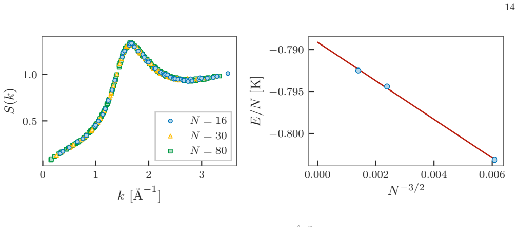
- Finite-size corrections scale as $N^{-1/2}$ for Bragg peak amplitudes and $N^{-3/2}$ for energies, so thermodynamic-limit extrapolation keeps the critical pressure near $0.53$ to $0.54\ \mathrm{K}\,\mathrm{\AA}^{-2}$.
Reading between the lines
- The $N=30$ continuous crossover could be interpreted as effective rounding of a first-order transition in a small box; one could test whether the crossover sharpens with additional variational freedom, which would confirm the finite-size reading.
- The same Gibbs-ensemble setup could measure the free-energy barrier between liquid and solid and estimate critical nucleus sizes, quantities the paper does not compute.
- A zero-temperature analog of the Kosterlitz-Thouless-Halperin-Nelson-Young scenario would predict algebraic hexatic order; the authors' data rule it out at $T=0$, but a finite-temperature extension of the same method could map the hexatic region above zero temperature.
- Entanglement entropy may serve as a sensitive order parameter for first-order quantum transitions in other bosonic or fermionic crystals.
Signed reviews
Editorial analysis
A structured set of objections, weighed in public.
Referee Report
Summary. The paper studies the zero-temperature phase diagram of two-dimensional helium-4 using a translation-invariant neural quantum state (NQS) in both canonical and isobaric variational Monte Carlo. The authors report a first-order superfluid-to-solid transition, with freezing and melting densities and a critical pressure, and argue that the apparent continuous crossover with hexatic order and a condensate fraction seen for N=30 is a finite-size artifact, since N=80 simulations exhibit metastable liquid and solid branches that support the Maxwell construction. They also compute the Rényi-2 entanglement entropy and observe a sharp drop at freezing. The main evidence is the constant-slope region in E(n), the abrupt density jump in isobaric runs, and the N=80 metastable branches; NQS energies are benchmarked against DMC in Table I.
Significance. If the conclusions hold, this is a valuable methodological and physical contribution: a single symmetric NQS functional form describes both liquid and solid without imposing symmetry, fixed-pressure NQS optimization allows cell-shape relaxation, and the paper makes concrete, falsifiable predictions for the coexistence densities and melting pressure. The DMC benchmarks and the variance reductions reported in Table I are strengths, as is the improved Rényi-2 estimator with random-origin averaging. The significance is tempered because the quantitative coexistence interval and the exclusion of a hexatic phase rest on N=80 metastable branches that are obtained by transfer learning and are not independently validated against the known phase-dependent variational bias; additional checks are needed before the phase diagram can be considered quantitative.
major comments (3)
- [Appendix C, Table I] The Maxwell construction in Appendix D uses spline fits to the N=80 liquid and solid branches, but Table I shows that the NQS energies on the N=80 solid branch are systematically above DMC by 14(3) mK at n=0.070 Å^-2 and 12(3) mK at n=0.075 Å^-2, while the N=80 liquid entries agree with DMC to within 1-3 mK at n=0.065 and 0.068 Å^-2. Because the solid branch anchors the high-density end of the common tangent, a constant upward bias of about 13 mK in the solid branch changes Pc by roughly δ/(n_m^-1 - n_f^-1) ≈ 0.018 KÅ^-2, which is comparable to the quoted 0.01 KÅ^-2 uncertainty and to the gap between the N=30 and N=80 pressure estimates. Please provide a bias-corrected Maxwell construction, for example by shifting the solid branch to the DMC energies, or otherwise demonstrate that the quoted coexistence interval and Pc are stable against this phase-dependent variational bias.
- [Appendix D, Fig. 7] The N=80 liquid and solid branches are generated by transfer learning from variational parameters optimized at deeper densities of the same phase, and no bidirectional initialization or unbiased optimization from the opposite phase is reported. In a translation-invariant ansatz, a solid is represented only if the Monte Carlo chain remains in a crystalline basin, so seeding from a solid-optimized state favors the solid branch by construction, and similarly for the liquid branch. This matters because the central finite-size argument for first-order melting and against a hexatic phase is precisely that N=80 exhibits two metastable branches while N=30 does not. Please demonstrate that each branch is a genuine local minimum at the relevant densities, for example by performing bidirectional sweeps (liquid initialization at densities above n_f and solid initialization below n_m) or by reporting order-parameter histograms and convergence from both initialization directions.
- [Main text and Appendices D/E] The paper reports materially different values for the critical pressure: 0.485(5) KÅ^-2 for N=30 in the isobaric ensemble (Fig. 1b), 0.50(1) KÅ^-2 for N=30 from canonical data (Appendix E), 0.53(1) KÅ^-2 for N=80 from the Maxwell construction, and 0.54(1) KÅ^-2 after finite-size extrapolation. The spread of about 0.04-0.05 KÅ^-2 is several times the quoted error bars. Since Pc and the coexistence interval are central quantitative predictions, please reconcile these values, state whether the discrepancy is due to finite-size effects, the ensemble, or the potential truncation, and report the N=30 and N=80 coexistence densities with the same definition. The statement in the Fig. 1 caption that the uncertainty on Pc is the pressure grid size appears to account only for grid resolution, not for statistical or variational uncertainty.
minor comments (4)
- [Appendix A and main text] Please state explicitly which potential form, the full periodized version of Eq. (A4) or the shifted and truncated version of Eq. (A8), is used for each figure and for the isobaric simulations; Table I and Fig. 8 clearly use the shifted and truncated potential, while the main-text equation of state does not specify this. This is necessary to reproduce the Pc values.
- [Figs. 2 and 4] The legends of Figs. 2 and 4 include N=56 data, but the text never discusses the N=56 results. Please state what the N=56 calculations add and whether they support the finite-size trend between N=30 and N=80.
- [Fig. 2] The 1/x fit f(x)=c1+c2(1/x+1/(min(L)-x)) is used to distinguish liquid from solid order, but the fitted values and uncertainties of c1 are not reported; giving them would make the liquid/solid distinction quantitative.
- [Eq. (2)] Please clarify the notation in the second exponential factor of Eq. (2): it is not clear whether the intended form is exp(-θ2/d_sin(ri,rj)^5) or exp(-θ2 d_sin(ri,rj)^5), and the definition of d_sin should be stated in the main text where Eq. (2) appears rather than only in Appendix B.
Circularity Check
No significant circularity: the phase diagram is obtained by minimizing a fixed Hamiltonian with DMC-benchmarked NQS energies and a standard Maxwell construction; self-citations concern methodology, not the physical conclusion.
full rationale
The paper's central claim—a first-order quantum liquid-to-solid transition in 2D 4He—is derived by minimizing the expectation value of a fixed microscopic Hamiltonian, Eq. (1), with the Aziz HFDHE2 potential (Appendix A), using neural quantum states. The energies entering the equation of state, the isobaric density jumps, and the Maxwell construction (Appendix D, Eqs. D1-D2) are computed observables, not fitted targets: the Maxwell construction is a thermodynamic identity applied to separately computed liquid and solid branch energies, not a parameter fitted to the transition. The same translation-invariant ansatz, Eq. (B2), is used for both phases, so no symmetry-breaking term or phase label is inserted that would force the transition; the N=30 crossover and N=80 metastable branches are emergent outcomes of variational optimization. Accuracy is independently checked against DMC in Table I, with NQS matching DMC to within 1-3 mK in the liquid and within 12-14 mK for the N=80 solid; this external benchmark means the physical conclusion does not reduce to the authors' prior universality claims. Self-citations to Refs. [51,52,73,74] concern the GNN/MP-NQS architecture and optimization methodology, not the existence or order of the transition, and are not used to forbid alternative phases. The skeptical objection about transfer-learned branches and variational bias is a concern about optimizer fidelity and finite-size extrapolation, not about definitional circularity; no equation in the paper defines the predicted transition in terms of the fit inputs. Therefore no circular step is established.
Assumptions & free parameters
free parameters (3)
- NQS variational parameters (theta1, theta2, MLP and GNN weights) =
optimized per density and phase; values not reported
- Spline fits l and s for liquid and solid energy branches =
nf=0.0681 Å^-2, nm=0.0716 Å^-2, Pc=0.53(1) KÅ^-2 for N=80
- Finite-size energy extrapolation parameters a and b =
b approximately -0.789 K at n=0.05 Å^-2; Pc_infinity=0.54(1) KÅ^-2
assumptions (6)
- domain assumption The Aziz HFDHE2 pair potential accurately describes helium-4 interactions.
- domain assumption Periodic boundary conditions with a shifted and truncated potential plus tail corrections reproduce bulk thermodynamics at these densities.
- domain assumption The neural quantum state ansatz is expressive enough to represent both liquid and solid ground states without imposed symmetry.
- standard math S(k) is linear in k at small k, implying N^-3/2 finite-size energy corrections.
- standard math The truncated swap estimator with random origin averaging gives unbiased Rényi-2 entropy estimates.
- domain assumption Transfer learning from deep liquid and solid optima yields true metastable branches rather than optimization artifacts.
Cite this review
Pith. "Pith review of Phase diagram and crystal melting of helium-4 in two dimensions." pith.science (2026). https://pith.science/paper/HZ7BADSZ
@misc{pith2026241205332,
  author       = {Pith},
  title        = {Pith review of: Phase diagram and crystal melting of helium-4 in two dimensions},
  year         = {2026},
  howpublished = {\url{https://pith.science/paper/HZ7BADSZ}},
  note         = {Machine review of arXiv:2412.05332}
}
abstract
We study the zero-temperature phase diagram of two-dimensional helium-4 using neural quantum states. Our variational description allows us to address liquid and solid phases using the same functional form as well as exploring possible melting scenarios, for instance via an intermediate hexatic phase. Notably, this is achieved by performing fixed pressure variational Monte Carlo calculations. Within the isobaric ensemble framework, we are able to clearly identify the first-order liquid-solid phase transition. However, in an intermediate region of nearly constant pressure, we find that simulations of $N=30$ atoms continuously transition from liquid to solid, with signatures of a hexatic order coexisting with a small condensate fraction. Calculations for larger systems follow the metastable liquid and solid branches in this transient region. We additionally compute the R\'enyi-2 entanglement entropy across the liquid-solid phase transition and find a sharp decrease upon freezing.
Figures


Figures from the paper (7 more)




Reference graph
Works this paper leans on
-
[1]
Kapitza, Nature141, 74 (1938)
P. Kapitza, Nature141, 74 (1938)
1938
-
[2]
J. F. Allen and A. D. Misener, Nature141, 75 (1938)
1938
-
[3]
London, Nature141, 643 (1938)
F. London, Nature141, 643 (1938)
1938
-
[4]
Landau, Phys
L. Landau, Phys. Rev.60, 356 (1941)
1941
-
[5]
N. N. Bogolyubov, J. Phys. (USSR)11, 23 (1947)
1947
-
[6]
R. P. Feynman, Phys. Rev.94, 262 (1954)
1954
-
[7]
Andreev and I
A. Andreev and I. Lifshitz, Sov. Phys. JETP29, 1107 (1969)
1969
-
[8]
Thouless, Annals of Physics52, 403 (1969)
D. Thouless, Annals of Physics52, 403 (1969)
work page 1969
Show all 88 references
-
[9]
A. J. Leggett, Phys. Rev. Lett.25, 1543 (1970)
1970
-
[10]
G. V. Chester, Phys. Rev. A2, 256 (1970)
1970
-
[11]
Boninsegni and N
M. Boninsegni and N. V. Prokof’ev, Rev. Mod. Phys.84, 759 (2012)
2012
-
[12]
Kim and M
E. Kim and M. H. W. Chan, Nature427, 225 (2004)
2004
-
[13]
Kim and M
E. Kim and M. H. W. Chan, Science305, 1941 (2004)
2004
-
[14]
Kim and M
E. Kim and M. H. W. Chan, Phys. Rev. Lett.97, 115302 (2006)
2006
-
[15]
D. M. Ceperley and B. Bernu, Phys. Rev. Lett. 93, 155303 (2004)
2004
-
[16]
B. K. Clark and D. M. Ceperley, Phys. Rev. Lett.96, 105302 (2006)
2006
-
[17]
Boninsegni, N
M. Boninsegni, N. Prokof’ev, and B. Svistunov, Phys. Rev. Lett.96, 105301 (2006)
2006
-
[18]
Boninsegni, A
M. Boninsegni, A. B. Kuklov, L. Pollet, N. V. Prokof’ev, B. V. Svistunov, and M. Troyer, Phys. Rev. Lett.97, 080401 (2006)
2006
-
[19]
D. Y. Kim and M. H. W. Chan, Phys. Rev. Lett.109, 155301 (2012)
2012
-
[20]
Beamish and S
J. Beamish and S. Balibar, Rev. Mod. Phys.92, 045002 (2020)
2020
-
[21]
Cinti, P
F. Cinti, P. Jain, M. Boninsegni, A. Micheli, P. Zoller, and G. Pupillo, Phys. Rev. Lett.105, 135301 (2010)
2010
-
[22]
Saccani, S
S. Saccani, S. Moroni, and M. Boninsegni, Phys. Rev. B 83, 092506 (2011)
2011
-
[23]
Saccani, S
S. Saccani, S. Moroni, and M. Boninsegni, Phys. Rev. Lett. 108, 175301 (2012)
2012
-
[24]
Böttcher, J.-N
F. Böttcher, J.-N. Schmidt, M. Wenzel, J. Hertkorn, M. Guo, T. Langen, and T. Pfau, Phys. Rev. X9, 011051 (2019)
2019
-
[25]
Chomaz, D
L. Chomaz, D. Petter, P. Ilzhöfer, G. Natale, A. Traut- mann, C. Politi, G. Durastante, R. M. W. van Bijnen, A. Patscheider, M. Sohmen, M. J. Mark, and F. Ferlaino, Phys. Rev. X9, 021012 (2019)
2019
-
[26]
Tanzi, E
L. Tanzi, E. Lucioni, F. Famà, J. Catani, A. Fioretti, C. Gabbanini, R. N. Bisset, L. Santos, and G. Modugno, Phys. Rev. Lett.122, 130405 (2019)
2019
-
[27]
Nakamura, K
S. Nakamura, K. Matsui, T. Matsui, and H. Fukuyama, Phys. Rev. B94, 180501 (2016)
2016
-
[28]
J. Choi, A. A. Zadorozhko, J. Choi, and E. Kim, Phys. Rev. Lett.127, 135301 (2021)
2021
-
[29]
J. M. Kosterlitz and D. J. Thouless, J. Phys. C6, 1181 (1973)
1973
-
[30]
B. I. Halperin and D. R. Nelson, Phys. Rev. Lett.41, 121 (1978)
1978
-
[31]
D. R. Nelson and B. I. Halperin, Phys. Rev. B19, 2457 (1979)
1979
-
[32]
A. P. Young, Phys. Rev. B19, 1855 (1979)
1979
-
[33]
E. P. Bernard and W. Krauth, Phys. Rev. Lett.107, 155704 (2011)
2011
-
[34]
S. C. Kapfer and W. Krauth, Phys. Rev. Lett. 114, 035702 (2015)
2015
-
[35]
Hajibabaei and K
A. Hajibabaei and K. S. Kim, Phys. Rev. E99, 022145 (2019)
2019
-
[36]
J. A. Anderson, J. Antonaglia, J. A. Millan, M. Engel, and S. C. Glotzer, Phys. Rev. X7, 021001 (2017)
2017
-
[37]
Apaja and M
V. Apaja and M. Saarela, Europhysics Letters84, 40003 (2008)
2008
-
[38]
long-range
combined with a deep layer structure in continuous space [39–42]. Using the same symmetric and trans- lationally invariant functional form, we are able to ac- curately describe phases of different spatial symmetries (liquid and solid), as well as the phenomena of Bose- Einstei...
2024 arXiv
-
[39]
Taddei, M
M. Taddei, M. Ruggeri, S. Moroni, and M. Holzmann, Phys. Rev. B91, 115106 (2015)
2015
-
[40]
Carleo and M
G. Carleo and M. Troyer, Science355, 602 (2017). 7
2017
-
[41]
Hermann, Z
J. Hermann, Z. Schätzle, and F. Noé, Nature Chemistry 12, 891 (2020)
2020
-
[42]
Holzmann and S
M. Holzmann and S. Moroni, Phys. Rev. B99, 085121 (2019)
2019
-
[43]
M. C. Gordillo and D. M. Ceperley, Phys. Rev. B58, 6447 (1998)
1998
-
[44]
D. Pfau, J. S. Spencer, A. G. Matthews, and W. M. C. Foulkes, Physical review research2, 033429 (2020)
2020
-
[45]
Krishnamachari and G
B. Krishnamachari and G. V. Chester, Phys. Rev. B61, 9677 (2000)
2000
-
[46]
Moroni, D
S. Moroni, D. E. Galli, S. Fantoni, and L. Reatto, Phys. Rev. B58, 909 (1998)
1998
-
[47]
M. C. Gordillo and J. Boronat, Phys. Rev. Lett.124, 205301 (2020)
2020
-
[48]
Arrigoni, E
F. Arrigoni, E. Vitali, D. E. Galli, and L. Reatto, Low Temperature Physics39, 793 (2013)
2013
-
[49]
R. A. Aziz, V. P. S. Nain, J. S. Carley, W. L. Taylor, and G. T. McConville, The Journal of Chemical Physics70, 4330 (1979)
1979
-
[50]
Boninsegni and S
M. Boninsegni and S. Moroni, Phys. Rev. B102, 235436 (2020)
2020
-
[51]
Pescia, J
G. Pescia, J. Nys, J. Kim, A. Lovato, and G. Carleo, Phys. Rev. B110, 035108 (2024)
2024
-
[52]
W. L. McMillan, Phys. Rev.138, A442 (1965)
1965
-
[53]
Ruggeri, S
M. Ruggeri, S. Moroni, and M. Holzmann, Phys. Rev. Lett. 120, 205302 (2018)
2018
-
[54]
Pescia, J
G. Pescia, J. Han, A. Lovato, J. Lu, and G. Carleo, Phys- ical Review Research4, 023138 (2022)
2022
-
[55]
N. M. Tubman and J. McMinis, Renyi entanglement en- tropy of molecules: Interaction effects and signatures of bonding (2012), arXiv:1204.4731 [cond-mat.str-el]
2012 arXiv
-
[56]
M. B. Hastings, I. González, A. B. Kallin, and R. G. Melko, Phys. Rev. Lett.104, 157201 (2010)
2010
-
[57]
C. M. Herdman, S. Inglis, P.-N. Roy, R. G. Melko, and A. D. Maestro, Physical Review E 90, 10.1103/phys- reve.90.013308 (2014)
2014 doi
-
[58]
McMinis and N
J. McMinis and N. M. Tubman, Physical Review B87, 10.1103/physrevb.87.081108 (2013)
2013 doi
-
[59]
Mauron, Z
L. Mauron, Z. Denis, J. Nys, and G. Carleo, Predict- ing topological entanglement entropy in a rydberg analog simulator (2024), arXiv:2406.19872 [quant-ph]
2024 arXiv
-
[60]
Sinibaldi, C
A. Sinibaldi, C. Giuliani, G. Carleo, and F. Vicentini, Quantum 7, 1131 (2023)
2023
-
[61]
Berezinskii, Sov
V. Berezinskii, Sov. Phys. JETP34, 610 (1972)
1972
-
[62]
D. J. Bishop and J. D. Reppy, Phys. Rev. Lett.40, 1727 (1978)
1978
-
[63]
Holzmann, R
M. Holzmann, R. C. Clay, M. A. Morales, N. M. Tubman, D. M. Ceperley, and C. Pierleoni, Physical Review B94, 10.1103/physrevb.94.035126 (2016)
2016 doi
-
[64]
around freezing densities. The isobaric ensem- ble methodological framework presented here, based on NQS, enables structural optimizations that can achieve diffusion Monte Carlo precision, which could be espe- cially relevant for electronic structure calculations. Acknowledgme...
-
[65]
J.M.Kosterlitz,JournalofPhysicsC:SolidStatePhysics 7, 1046 (1974)
1974
-
[66]
J. P. Toennies, A. F. Vilesov, and K. B. Whaley, Physics Today54, 31 (2001)
2001
-
[67]
Carleo, K
G. Carleo, K. Choo, D. Hofmann, J. E. Smith, T. Wester- hout, F. Alet, E. J. Davis, S. Efthymiou, I. Glasser, S.-H. Lin, M.Mauri, G.Mazzola, C.B.Mendl, E.vanNieuwen- burg, O. O’Reilly, H. Théveniaut, G. Torlai, F. Vicentini, and A. Wietek, SoftwareX10, 100311 (2019)
2019
-
[68]
Vicentini, D
F. Vicentini, D. Hofmann, A. Szabó, D. Wu, C. Roth, C. Giuliani, G. Pescia, J. Nys, V. Vargas-Calderón, N. Astrakhantsev, and G. Carleo, SciPost Phys. Code- bases , 7 (2022)
2022
-
[69]
Bradbury, R
J. Bradbury, R. Frostig, P. Hawkins, M. J. Johnson, C. Leary, D. Maclaurin, G. Necula, A. Paszke, J. Van- derPlas, S. Wanderman-Milne, and Q. Zhang, JAX: com- posable transformations of Python+NumPy programs (2018)
2018
-
[70]
Häfner and F
D. Häfner and F. Vicentini, Journal of Open Source Soft- ware 6, 3419 (2021)
2021
-
[71]
M. V. den Nest, Simulating quantum computers with probabilistic methods (2010), arXiv:0911.1624 [quant- ph]
2010 arXiv
-
[72]
J. E. Kilpatrick, W. E. Keller, E. F. Hammel, and N. Metropolis, Phys. Rev.94, 1103 (1954)
1954
-
[73]
K. S. Liu, M. H. Kalos, and G. V. Chester, Phys. Rev. B 13, 1971 (1976)
1976
-
[74]
Frenkel and B
D. Frenkel and B. Smit,Understanding Molecular Sim- ulation: From Algorithms to Applications , 2nd ed. (Aca- demic Press, San Diego, CA, 2002)
2002
-
[75]
J. Kim, G. Pescia, B. Fore, J. Nys, G. Carleo, S. Gan- dolfi, M. Hjorth-Jensen, and A. Lovato, Communications Physics 7, 148 (2024)
2024
-
[76]
J. Nys, G. Pescia, A. Sinibaldi, and G. Carleo, Nature Communications 15, 9404 (2024)
2024
-
[77]
Gilmer, S
J. Gilmer, S. S. Schoenholz, P. F. Riley, O. Vinyals, and G. E. Dahl, Neural message passing for quantum chem- istry (2017)
2017
-
[78]
Vaswani, N
A. Vaswani, N. Shazeer, N. Parmar, J. Uszkoreit, L. Jones, A. N. Gomez, L. Kaiser, and I. Polosukhin, Attention is all you need (2017)
2017
-
[79]
Veličković, G
P. Veličković, G. Cucurull, A. Casanova, A. Romero, P. Liò, and Y. Bengio, Graph attention networks (2018), arXiv:1710.10903
2018 arXiv
-
[80]
P. W. Battaglia, J. B. Hamrick, V. Bapst, A. Sanchez- Gonzalez, V. Zambaldi, M. Malinowski, A. Tacchetti, D. Raposo, A. Santoro, R. Faulkner, C. Gulcehre, F. Song, A. Ballard, J. Gilmer, G. Dahl, A. Vaswani, K. Allen, C. Nash, V. Langston, C. Dyer, N. Heess, D. Wierstra, P. Ko...
2018 arXiv
-
[81]
Boninsegni and S
M. Boninsegni and S. Moroni, Phys. Rev. E86, 056712 (2012)
2012
-
[82]
Chiesa, D
S. Chiesa, D. M. Ceperley, R. M. Martin, and M. Holz- mann, Phys. Rev. Lett.97, 076404 (2006)
2006
-
[83]
Feenberg, Theory of Quantum Fluids , Pure and ap- plied physics (Academic Press, 2012)
E. Feenberg, Theory of Quantum Fluids , Pure and ap- plied physics (Academic Press, 2012). 8 SUPPLEMENTAL MATERIAL Appendix A: Helium potential energy under periodic boundary conditions We use the Aziz HFDHE2 pair potential [49] to model the interatomic interactions between he...
2012
-
[84]
Periodized potential The full periodized potential reads V (R) = 1 2 X i,j X n ′ v(|rij + nL|), (A4) where v(r) ≡ vAziz(r/rm), rij = ri − rj is the distance vector between particlei and particle j, L = (Lx, Ly) is the size of the simulation cell, and the restriction on the sum...
-
[85]
In this case, the full potential energy V (R) can be written as follows V (R) = Vs + Vt + X i<j ˜v(rij), (A8) where only the third term depends on the Monte Carlo samples
Shifted and truncated potential Instead of considering all periodic images (up to a chosen cutoff), as in Appendix A1, the potential can be restricted to account for only a single image, provided corrections are taken into account. In this case, the full potential energy V (R)...
-
[86]
Here we will focus on the case where the 18 full system is in a pure quantum state|Ψ⟩, so that the density matrix isρ = |Ψ⟩⟨Ψ|/⟨Ψ|Ψ⟩
Standard swap estimator Given two partitions A and B of a physical system, the reduced density matrix of subsystem A is obtained via ρA = TrBρ, that is, by tracing out the degrees of freedom of subsystem B. Here we will focus on the case where the 18 full system is in a pure q...
-
[87]
We also denote the metric of integration bydΩ ≡ dRAdR′ AdRBdR′ B
Truncated swap estimator To simplify notation, we letx1 ≡ RA ∪ RB, x2 ≡ R′ A ∪ R′ B, y1 ≡ R′ A ∪ RB and y2 ≡ RA ∪ R′ B. We also denote the metric of integration bydΩ ≡ dRAdR′ AdRBdR′ B. Eq. (H6) can then be written more compactly as follows TrAρ2 A = Z dΩΨ∗(x1)Ψ∗(x2)Ψ(y1)Ψ(y2)...
-
[88]
Periodic systems and random origins Periodic systems do not have a preferred origin. As a result, for each Monte Carlo sample, we randomly displace the center of partition A in the simulation cell, denotedC ≡[0, Lx] × [0, Ly], to calculate different instances of the TrAρ2 A es...
Reviewed August 11, 2026 · model on record in the stance chip above.
Discussion (0). Continue with ORCID to comment.