REVIEW 2 major objections 5 minor 36 references
Causal Effect Identification in Heterogeneous Environments from Higher-Order Moments
T0 review · 2 major / 5 minor · reviewed 2026-08-07 · deepseek-v4-flash
Pith's one-line read Given two environments that differ in exactly one causal parameter, the treatment effect β can be recovered from higher-order moments: uniquely when the change is in a path coefficient, and up to two candidates when the change is in a…
desk verdict Useful four-way identifiability map for a two-environment linear confounding triangle, but the proofs rely on an unstated zero-mean noise assumption that the experiments also violate. read the letter →
The pith
A machine-rendered reading of the paper's core claim, the machinery that carries it, and where it could break.
The reading
What carries the argument
The load-bearing object is a family of ratio identities built from cross-moments. For example, when only ϵt varies, the first moment k where the two noise distributions differ gives β = (E[Y⁽¹⁾(T⁽¹⁾)^{k−1}] − E[Y⁽²⁾(T⁽²⁾)^{k−1}]) / (E[(T⁽¹⁾)^k] − E[(T⁽²⁾)^k]), because all invariant terms cancel. The same difference-and-divide device is adapted to each of the four cases, with the cross-moment subroutine GetRatio recovering coefficient ratios such as γ/α from variables that share a common latent term. The non-identifiability proof uses an explicit reconstruction that swaps αϵu with ϵt and replaces γ with −γ/α, producing identical observed distributions with a different β.
What would settle it
Run Algorithm 1 on two environments generated with only ϵt changing, all noises drawn from uncentered exponential distributions with different rates; if the estimate does not approach the true β as sample size grows, the zero-mean premise is necessary and the stated identifiability result is incomplete.
Extended reading notes
Core claim
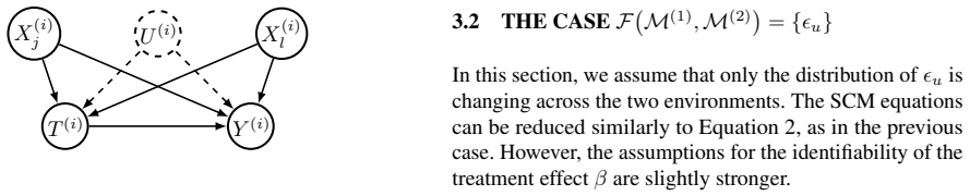
On the paper's own terms, the central discovery is Theorem 3.1: for two linear structural causal models compatible with U→T, U→Y, and T→Y, if exactly one non-outcome parameter or noise distribution differs across environments, β is identifiable—uniquely when the difference is in α or γ, and up to two candidates when it is in ϵt or ϵu. Theorems 3.2–3.5 give constructive moment formulas and algorithms for each case, and Theorem 3.6 shows that if both ϵu and ϵt vary, two observationally equivalent SCMs with different β exist, so identifiability fails. The uniqueness cases require a mild non-Gaussianity condition, namely some n with E[ϵⁿ] ≠ (n−1)E[ϵⁿ⁻²]E[ϵ²]. The paper further claims a detection step, based on second moments, that locates the varying parameter and leaves only the ϵt-versus-ϵu distinction unresolved.
Load-bearing premise
The theorems assume both that exactly one mechanism varies and that every exogenous noise has zero mean, the latter being unstated in Assumptions 1–4; if either fails, the ratio estimators are no longer guaranteed to recover β.
Editorial extensions
If this is right
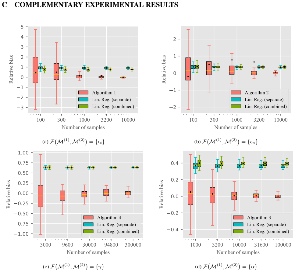
- Given knowledge of which single parameter changed, Algorithms 1–4 estimate β consistently as sample size grows, while ordinary least-squares baselines remain systematically biased.
- A change in α or γ identifies the causal effect exactly; a change in ϵt or ϵu leaves only two candidates, so the ambiguity is finite and searchable.
- The Section 3.5 detection procedure distinguishes γ, α, and the noise cases from observed second moments alone; only the ϵt-versus-ϵu distinction is unresolvable.
- If both ϵu and ϵt vary across environments, two environments cannot identify β at all, regardless of sample size.
- Observed covariates can be absorbed by residualization, and more than two environments can be handled pairwise, making the two-environment analysis the core building block.
Reading between the lines
- A practitioner who runs the full pipeline and finds two candidate effects should treat the ϵt/ϵu ambiguity as a real modeling choice; a third environment with a different kind of shift is the natural way to break the tie.
- Every proof cancels terms using zero-mean noises, so the effective theorem includes an unstated zero-mean condition; centering the data before applying the algorithms is a cheap, testable fix.
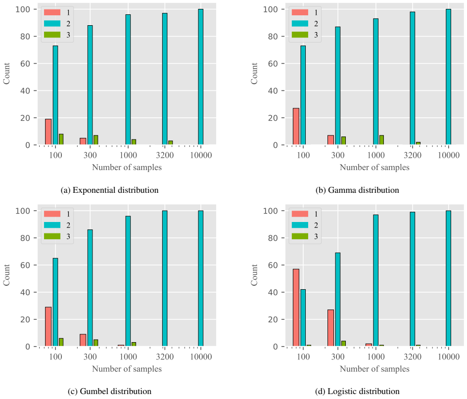
- Because the algorithms need only the first moment index k where the changing distributions differ, they can be run without knowing the noise family, and the paper's histograms suggest k is usually small for common distributions.
Editorial analysis
A structured set of objections, weighed in public.
Referee Report
Summary. The paper studies the problem of estimating the causal effect β of treatment T on outcome Y in a linear structural causal model with a latent confounder U, using observational data from two environments. Under the assumption that exactly one of the coefficients α, γ or one of the exogenous noises ε_t, ε_u varies across environments, the authors propose moment-based estimators (Algorithms 1–4) and prove that β is uniquely identifiable when the change is in α or γ, and identifiable up to two candidates when the change is in ε_t or ε_u. They also prove a non-identifiability result when both ε_u and ε_t vary, and provide a procedure to detect the source of the change. The paper reports synthetic experiments with exponential, Gamma, Gumbel, and Logistic noises.
Significance. The paper addresses a timely and relevant problem: estimating a causal effect under latent confounding when data come from multiple environments with a single unknown source of heterogeneity. The constructive moment-based estimators and the explicit non-identifiability theorem are useful contributions, and the paper is careful in distinguishing cases where β is uniquely identifiable from cases where only a finite set of candidates can be recovered. The reliance on the GetRatio subroutine from prior work is clearly flagged. If the zero-mean gap described in the major comments is fixed by amending the assumptions and adjusting the experiments, the results would be a valuable addition to the multi-environment causal inference literature.
major comments (2)
- [Assumptions 1–4 and Appendix A (Eqs. (10), (13), (24)–(25))] The proofs of Theorems 3.2–3.5 and the change-detection tests in Section 3.5 rely on the assumption that all exogenous noises have zero mean, but Assumptions 1–4 never state this. For instance, in the proof of Theorem 3.2, Eq. (10) drops terms involving E[ε_y] by stating that 'the exogenous noises are independent and mean zero.' If the means are nonzero, the ratio in Algorithm 1 is biased; analogous biases appear in Algorithms 2–4 and in the detection ratios of Section 3.5. For the γ case, letting μ_u=E[ε_u], μ_t=E[ε_t], μ_y=E[ε_y], the quantity computed in Algorithm 4, line 1, equals 2β+γ1+γ2 + [2μ_u μ_y − (γ1+γ2) μ_u μ_t]/[E[ε_u^2]+μ_u μ_t], not the claimed 2β+γ1+γ2. This is load-bearing: the estimators and classification procedure are not correct for the model class defined by Assumptions 1–4. The authors should either add a zero-mean assumption to the theorems, or modify the estimators/detection rules to account for nonzero means.
- [Section 5 (Experiments)] The experiments in Section 5 sample all noise variables from an exponential distribution with rate λ ∈ (0.9, 1.1), and the text does not mention centering. Exponential noises have mean 1/λ, so the data used in Figures 4–11 do not satisfy the (unstated) zero-mean condition under which the estimators are proven. As a result, the reported convergence of the algorithms does not validate the theorems as stated. The authors should either center the noises in the experimental protocol, add the zero-mean assumption to the theorems, or clearly report and justify the experimental regime, and then re-run or re-describe the simulations accordingly.
minor comments (5)
- [Theorem 3.1 vs. Theorem 3.5] Theorem 3.1 states that β is uniquely identified when F⊂{α,γ}, but the α case in Theorem 3.5 holds only 'almost surely' with respect to Lebesgue measure on coefficients; this qualifier should appear in Theorem 3.1 and the abstract.
- [Section 3.3, Step 5, Case 2] The expression 'ϕ(1)n∗ − ϕ(1)n∗ = 0' appears to be a typo; it should read 'ϕ(1)n∗ − ϕ(2)n∗ = 0', and likewise 'ϕ(1)n∗ + ϕ(1)n∗ ≠ 0' should read 'ϕ(1)n∗ + ϕ(2)n∗ ≠ 0'.
- [Algorithm 3 (Section 3.4)] Algorithm 3 has input 'F(M(1),M(2)) = {ϵt}', but the algorithm is for the α case and the input should be '{α}'.
- [Figure 4 caption] In Figure 4 (and similarly in Figures 5–11), the caption for panel (b) repeats 'only ϵt'; it should be 'only ϵu'.
- [Throughout] The paper should explicitly state that α≠0 and γ≠0, since several steps divide by these coefficients (e.g., the rescaling in Section 3.3 and the construction in Theorem 3.6).
Circularity Check
No significant circularity: the moment-ratio estimators are derived by direct algebra, and the cited subroutines (GetRatio, external counterexample) are not restatements of the target effect.
full rationale
The central derivation is not circular. Theorem 3.2's proof expands E[Y(T)^{k-1}] and E[T^k] in terms of noise moments and cancels invariant terms, giving beta directly as a ratio of observable moments (Eq. (11)); this is closed-form algebra, not a fitted parameter. Theorems 3.3-3.5 and Algorithms 2-4 similarly derive moment identities; the only imported subroutine is GetRatio from the authors' prior work (Kivva et al., 2024), used to recover gamma/alpha from a pair of variables sharing a hidden component. That is a cited external lemma with its own assumptions, not a restatement of the target beta, and the non-identifiability result (Theorem 3.6) uses an external counterexample from Salehkaleybar et al. (2020). The proofs do rely on an unstated zero-mean noise premise, for example Eq. (10) says 'exogenous noises are independent and mean zero' although Assumptions 1-4 do not state it, and the experiments use uncentered exponential noise; this is an omitted-assumption/correctness gap, not a circular reduction, because the moment formulas are not defined in terms of the quantity they estimate. The Appendix's admission that Algorithm 3 can use an incorrect n for logistic noise at small sample sizes is likewise an acknowledged limitation, not a circular step. No step was found in which an input is defined by the output or a prediction equals a fit by construction.
Assumptions & free parameters
assumptions (8)
- domain assumption Linear SCM: each variable is a linear function of its parents plus exogenous noise (Assumption 1)
- domain assumption Causal effect invariance: beta is identical across environments (Assumption 2)
- domain assumption Finite moments of all orders (Assumption 3)
- domain assumption Distributions determined by moments (Assumption 4)
- ad hoc to paper Exogenous noises have zero mean
- domain assumption Exactly one parameter or noise distribution varies between the two environments (|F|=1)
- domain assumption Non-Gaussianity of epsilon_t (in Theorems 3.3 and 3.4) or of epsilon_u (in Theorem 3.5)
- ad hoc to paper alpha != 0 and gamma != 0 for rescaling and ratios
Cite this review
Pith. "Pith review of Causal Effect Identification in Heterogeneous Environments from Higher-Order Moments." pith.science (2026). https://pith.science/paper/I25SB2O2
@misc{pith2026250611756,
  author       = {Pith},
  title        = {Pith review of: Causal Effect Identification in Heterogeneous Environments from Higher-Order Moments},
  year         = {2026},
  howpublished = {\url{https://pith.science/paper/I25SB2O2}},
  note         = {Machine review of arXiv:2506.11756}
}
read the original abstract
We investigate the estimation of the causal effect of a treatment variable on an outcome in the presence of a latent confounder. We first show that the causal effect is identifiable under certain conditions when data is available from multiple environments, provided that the target causal effect remains invariant across these environments. Secondly, we propose a moment-based algorithm for estimating the causal effect as long as only a single parameter of the data-generating mechanism varies across environments -- whether it be the exogenous noise distribution or the causal relationship between two variables. Conversely, we prove that identifiability is lost if both exogenous noise distributions of both the latent and treatment variables vary across environments. Finally, we propose a procedure to identify which parameter of the data-generating mechanism has varied across the environments and evaluate the performance of our proposed methods through experiments on synthetic data.
Figures


Figures from the paper (13 more)





Reference graph
Works this paper leans on
-
[1]
Joshua D Angrist and Alan B Krueger. Does compulsory school attendance affect schooling and earnings? The Quarterly Journal of Economics, 106 0 (4): 0 979--1014, 1991
work page 1991
-
[2]
Martin Arjovsky, L \'e on Bottou, Ishaan Gulrajani, and David Lopez-Paz. Invariant risk minimization. arXiv preprint arXiv:1907.02893, 2019
arXiv 1907
-
[3]
Meta-Learned Invariant Risk Minimization
Jun-Hyun Bae, Inchul Choi, and Minho Lee. Meta-learned invariant risk minimization. arXiv preprint arXiv:2103.12947, 2021
work page Pith review arXiv 2021
-
[4]
Transportability from multiple environments with limited experiments: Completeness results
Elias Bareinboim and Judea Pearl. Transportability from multiple environments with limited experiments: Completeness results. Advances in neural information processing systems, 27, 2014
work page 2014
-
[5]
Differentiable causal discovery from interventional data
Philippe Brouillard, S \'e bastien Lachapelle, Alexandre Lacoste, Simon Lacoste-Julien, and Alexandre Drouin. Differentiable causal discovery from interventional data. Advances in Neural Information Processing Systems, 33: 0 21865--21877, 2020
work page 2020
-
[6]
Invariance, causality and robustness
Peter B \"u hlmann. Invariance, causality and robustness. Statistical Science, 35 0 (3): 0 404--426, 2020
work page 2020
-
[7]
Minimum wages and employment: A case study of the fast food industry in new jersey and pennsylvania
David Card. Minimum wages and employment: A case study of the fast food industry in new jersey and pennsylvania. American Economic Review, 1993
work page 1993
-
[8]
Learning causal structures using regression invariance
AmirEmad Ghassami, Saber Salehkaleybar, Negar Kiyavash, and Kun Zhang. Learning causal structures using regression invariance. Advances in Neural Information Processing Systems, 30, 2017
work page 2017
Show all 36 references
-
[9]
Identifying invariant factors across multiple environments with kl regression
Jaime Roquero Gimenez and James Zou. Identifying invariant factors across multiple environments with kl regression. arXiv preprint arXiv:2002.08341, 2020
2002 arXiv
-
[10]
a gele, Jonas Rothfuss, Lars Lorch, Vignesh Ram Somnath, Bernhard Sch \
Alexander H \"a gele, Jonas Rothfuss, Lars Lorch, Vignesh Ram Somnath, Bernhard Sch \"o lkopf, and Andreas Krause. Bacadi: Bayesian causal discovery with unknown interventions. In International Conference on Artificial Intelligence and Statistics, pages 1411--1436. PMLR, 2023
2023
-
[11]
Invariant causal prediction for nonlinear models
Christina Heinze-Deml, Jonas Peters, and Nicolai Meinshausen. Invariant causal prediction for nonlinear models. Journal of Causal Inference, 6 0 (2): 0 20170016, 2018
2018
-
[12]
Causal discovery from heterogeneous/nonstationary data
Biwei Huang, Kun Zhang, Jiji Zhang, Joseph Ramsey, Ruben Sanchez-Romero, Clark Glymour, and Bernhard Sch \"o lkopf. Causal discovery from heterogeneous/nonstationary data. Journal of Machine Learning Research, 21 0 (89): 0 1--53, 2020
2020
-
[13]
Causal inference in the social sciences
Guido W Imbens. Causal inference in the social sciences. Annual Review of Statistics and Its Application, 11, 2024
2024
-
[14]
Causal discovery from soft interventions with unknown targets: Characterization and learning
Amin Jaber, Murat Kocaoglu, Karthikeyan Shanmugam, and Elias Bareinboim. Causal discovery from soft interventions with unknown targets: Characterization and learning. Advances in neural information processing systems, 33: 0 9551--9561, 2020
2020
-
[15]
A cross-moment approach for causal effect estimation
Yaroslav Kivva, Saber Salehkaleybar, and Negar Kiyavash. A cross-moment approach for causal effect estimation. Advances in Neural Information Processing Systems, 36, 2024
2024
-
[16]
General transportability--synthesizing observations and experiments from heterogeneous domains
Sanghack Lee, Juan Correa, and Elias Bareinboim. General transportability--synthesizing observations and experiments from heterogeneous domains. In Proceedings of the AAAI Conference on Artificial Intelligence, volume 34, pages 10210--10217, 2020
2020
-
[17]
Nonlinear invariant risk minimization: A causal approach
Chaochao Lu, Yuhuai Wu, Jo \'s e Miguel Hern \'a ndez-Lobato, and Bernhard Sch \"o lkopf. Nonlinear invariant risk minimization: A causal approach. arXiv preprint arXiv:2102.12353, 2021
2021 arXiv
-
[18]
Learning causal models under independent changes
Sarah Mameche, David Kaltenpoth, and Jilles Vreeken. Learning causal models under independent changes. Advances in Neural Information Processing Systems, 36, 2024
2024
-
[19]
Joint causal inference from multiple contexts
Joris M Mooij, Sara Magliacane, and Tom Claassen. Joint causal inference from multiple contexts. Journal of machine learning research, 21 0 (99): 0 1--108, 2020
2020
-
[20]
Causality
Judea Pearl. Causality. Cambridge university press, 2009
2009
-
[21]
Probabilistic reasoning in intelligent systems: networks of plausible inference
Judea Pearl. Probabilistic reasoning in intelligent systems: networks of plausible inference. Elsevier, 2014
2014
-
[22]
u gelgen, and Bernhard Sch \
Ronan Perry, Julius Von K \"u gelgen, and Bernhard Sch \"o lkopf. Causal discovery in heterogeneous environments under the sparse mechanism shift hypothesis. Advances in Neural Information Processing Systems, 35: 0 10904--10917, 2022
2022
-
[23]
Causal inference by using invariant prediction: identification and confidence intervals
Jonas Peters, Peter B \"u hlmann, and Nicolai Meinshausen. Causal inference by using invariant prediction: identification and confidence intervals. Journal of the Royal Statistical Society Series B: Statistical Methodology, 78 0 (5): 0 947--1012, 2016
2016
-
[24]
Invariant causal prediction for sequential data
Niklas Pfister, Peter B \"u hlmann, and Jonas Peters. Invariant causal prediction for sequential data. Journal of the American Statistical Association, 114 0 (527): 0 1264--1276, 2019
2019
-
[25]
Marginal structural models and causal inference in epidemiology, 2000
James M Robins, Miguel Angel Hernan, and Babette Brumback. Marginal structural models and causal inference in epidemiology, 2000
2000
-
[26]
The central role of the propensity score in observational studies for causal effects
Paul R Rosenbaum and Donald B Rubin. The central role of the propensity score in observational studies for causal effects. Biometrika, 70 0 (1): 0 41--55, 1983
1983
-
[27]
a usler, Peter B \
Dominik Rothenh \"a usler, Peter B \"u hlmann, and Nicolai Meinshausen. Causal dantzig. The Annals of Statistics, 47 0 (3): 0 1688--1722, 2019
2019
-
[28]
a usler, Nicolai Meinshausen, Peter B \
Dominik Rothenh \"a usler, Nicolai Meinshausen, Peter B \"u hlmann, and Jonas Peters. Anchor regression: Heterogeneous data meet causality. Journal of the Royal Statistical Society Series B: Statistical Methodology, 83 0 (2): 0 215--246, 2021
2021
-
[29]
Learning linear non-gaussian causal models in the presence of latent variables
Saber Salehkaleybar, AmirEmad Ghassami, Negar Kiyavash, and Kun Zhang. Learning linear non-gaussian causal models in the presence of latent variables. Journal of Machine Learning Research, 21 0 (39): 0 1--24, 2020
2020
-
[30]
Causal discovery of linear non-gaussian causal models with unobserved confounding
Daniela Schkoda, Elina Robeva, and Mathias Drton. Causal discovery of linear non-gaussian causal models with unobserved confounding. arXiv preprint arXiv:2408.04907, 2024
2024 arXiv
-
[31]
Invariant representation learning for treatment effect estimation
Claudia Shi, Victor Veitch, and David M Blei. Invariant representation learning for treatment effect estimation. In Uncertainty in artificial intelligence, pages 1546--1555. PMLR, 2021
2021
-
[32]
Permutation-based causal structure learning with unknown intervention targets
Chandler Squires, Yuhao Wang, and Caroline Uhler. Permutation-based causal structure learning with unknown intervention targets. In Conference on Uncertainty in Artificial Intelligence, pages 1039--1048. PMLR, 2020
2020
-
[33]
Causal invariance learning via efficient optimization of a nonconvex objective
Zhenyu Wang, Yifan Hu, Peter B \"u hlmann, and Zijian Guo. Causal invariance learning via efficient optimization of a nonconvex objective. arXiv preprint arXiv:2412.11850, 2024
2024
-
[34]
Optimization-based causal estimation from heterogeneous environments
Mingzhang Yin, Yixin Wang, and David M Blei. Optimization-based causal estimation from heterogeneous environments. J. Mach. Learn. Res, 25: 0 1--44, 2024
2024
-
[35]
Invariant causal prediction for block mdps
Amy Zhang, Clare Lyle, Shagun Sodhani, Angelos Filos, Marta Kwiatkowska, Joelle Pineau, Yarin Gal, and Doina Precup. Invariant causal prediction for block mdps. In International Conference on Machine Learning, pages 11214--11224. PMLR, 2020
2020
-
[36]
Causal discovery with heterogeneous observational data
Fangting Zhou, Kejun He, and Yang Ni. Causal discovery with heterogeneous observational data. In Uncertainty in Artificial Intelligence, pages 2383--2393. PMLR, 2022
2022
Reviewed August 7, 2026 · model on record in the stance chip above.
Discussion (0). Continue with ORCID to comment.