Charged cosmological black holes: a thorough study of a family of solutions

Alan Maciel; Daniel C. Guariento; Marina M. C. Mello; Vilson T. Zanchin

REVIEW 3 major objections 5 minor 67 references

Charged cosmological black holes: a thorough study of a family of solutions

T0 review · 3 major / 5 minor · reviewed 2026-08-14 · deepseek-v4-flash

Challenge this review Re-run · record.json Download PDF Read on arXiv ↗ Review JSON

Pith's one-line read A charged cousin of the McVittie cosmological black hole is shown to be an exact Einstein–Maxwell–cuscuton solution with four distinct causal structures, including naked singularities.

desk verdict A careful, mostly explicit exact-solution classification whose headline causal-structure theorem is stated more strongly than it is proved. read the letter →

arxiv 1908.04961 v2 pith:IEBQBP4D submitted 2019-08-14 gr-qc hep-th

Daniel C. Guariento , Alan Maciel , Marina M. C. Mello , Vilson T. Zanchin This is my paper · ORCID

classification gr-qchep-th MSC 83C5783C1583C75 PACS 04.40.-b04.20.Jb04.70.-s04.70.Bw

keywords Shah–VaidyasolutionchargedMcVittiespacetimecuscutonfieldapparenthorizonsnakedsingularitycausalstructureEinstein–MaxwellequationsReissner–Nordström–deSitter

verification ladder T0 review T1 audit T2 compute T3 formal

The pith

A machine-rendered reading of the paper's core claim, the machinery that carries it, and where it could break.

The reading

The paper establishes that the Shah–Vaidya metric, the charged, time-dependent cousin of McVittie's cosmological black hole, is an exact solution of the Einstein–Maxwell equations sourced by a neutral cuscuton field, with the cuscuton potential fixed by consistency. It then classifies all causal structures the metric allows under a few assumptions about the Hubble rate, finding four regions in parameter space governed by $q^2/m^2$ and $mH(t)$: two, zero, three, or one apparent horizons. Undercharged cases mirror the uncharged McVittie spacetime, while overcharged cases can develop naked timelike singularities at $R=0$. A stated theorem, extending the McVittie result, determines whether the late-time continuation joins the Reissner–Nordström–de Sitter limit as a single black hole or as a black-hole/white-hole pair, depending on how fast $H(t)$ approaches its asymptotic value. This matters because it turns a metric known since 1968 into a fully sourced model and gives a parameter map for when a charged cosmological black hole is well behaved and when it is not.

What carries the argument

The load-bearing object is the Shah–Vaidya metric written in areal-radius coordinates, $ds^2 = -N^2 dt^2 + (dR/N - HR\,dt)^2 + R^2 d\Omega^2$, with lapse $N(R) = \sqrt{1 - 2m/R + q^2/R^2}$. The causal classification reduces to the quartic $P(x) = h^2 x^4 - x^2 + 2x - \sigma^2$, whose positive roots are the apparent horizons; the extremal boundaries where roots coalesce come from $P'(x) = 0$ and give closed curves $\sigma^2_{c\pm}(h)$. A second mechanism is the coordinate $\tau$ used to glue the metric at future timelike infinity to a Reissner–Nordström–de Sitter patch, whose convergence is controlled by integrals $F_\pm$ of $e^{(B \pm \delta)u}\Delta H(u)$; this is the same machine as the uncharged McVittie causal-structure theorem.

What would settle it

Construct the maximal analytic extension of the undercharged Shah–Vaidya metric and check whether the surface $R = R_+$ is a genuine curvature singularity or a removable boundary; if extension is possible with finite curvature scalars, the claim that the physical spacetime ends at $R_+$ is false and the causal diagrams for Regions I and II would need revision.

Watch

Extended reading notes

Core claim

The central discovery is that the Shah–Vaidya metric is not just a generalization of McVittie's spacetime but a genuine solution of the coupled Einstein–Maxwell–cuscuton system, with the cuscuton potential fixed to $V = 3\mu^4/[4(\varphi - V_0)^2]$, and that its causal structure is governed by the dimensionless pair $(\sigma^2, h) = (q^2/m^2, mH(t))$. Solving the apparent-horizon condition $h^2 x^4 - x^2 + 2x - \sigma^2 = 0$ yields four parameter regions: Region I has two apparent horizons, Region II has none and exposes a naked singularity, Region III has three horizons, and Region IV has one. In undercharged cases the singularity at $R = R_+$ is spacelike and the outer region behaves like the uncharged McVittie case; in overcharged cases the only curvature singularity is at $R = 0$ and is timelike, so observers can see it. The paper further states a proposition that decides, from the late-time decay of $H(t)$, whether the spacetime extends into a single Reissner–Nordström–de Sitter black hole or into a black-hole/white-hole pair.

Load-bearing premise

The whole causal classification assumes that the discarded coordinate patches below $R = R_+$ (or below $R = m$ in the extremal case) are not part of the spacetime; if a maximal extension connects those patches to the main region, the global causal structure would differ from the diagrams shown.

Editorial extensions

If this is right

Undercharged Shah–Vaidya spacetimes that asymptote to Reissner–Nordström–de Sitter admit exactly the two causal structures found for uncharged McVittie, a single black hole or a black-hole/white-hole pair, selected by how $H(t)$ approaches its late-time constant.
Slightly overcharged cases with $1 < q^2/m^2 < 9/8$ can have three apparent horizons and a naked timelike singularity at $R=0$, a structure that does not exist in the uncharged McVittie solution.
Strongly overcharged cases, or cases with large $mH(t)$, form only one apparent horizon and leave the $R=0$ singularity visible to external observers.
If $H(t) \to 0$ at late times, the spacetime asymptotes to the Reissner–Nordström solution and inherits its causal skeleton: two horizons when $m^2 > q^2$ and one horizon when $m^2 < q^2$.
Because the metric is derived from an explicit action rather than imposed by hand, the mass and charge parameters come with a concrete physical source, a neutral cuscuton plus an electromagnetic field, so the solution can be used as a testbed for charged collapse in expanding backgrounds.

Reading between the lines

Editorial extensions of the paper, not claims the author makes directly.

The four-region horizon diagram may apply beyond this exact metric: any shear-free, spherically symmetric charged cosmological solution with the same algebraic horizon condition will share the same qualitative causal map, so the classification could serve as a template for other charged dynamical black holes.
Since the cuscuton field is non-dynamical, the Shah–Vaidya metric should be generic inside a larger family of Einstein–Maxwell–scalar models; one testable extension is to check whether adding a small dynamical scalar perturbation preserves the horizon count or shifts the extremal curves $\sigma^2_{c\pm}(h)$.
The paper shows that when $\Delta H(t)$ decays slower than $e^{-Bt}$, the chosen $\tau$ coordinate fails to glue the extension, but geodesic incompleteness without a singularity still suggests some other extension exists; constructing that extension would settle whether the naked timelike singularity persists in the global spacetime.
A numerical simulation of charged spherical collapse in a cuscuton background could test which parameter regions are dynamically reached from regular initial data, connecting the classification to astrophysical formation scenarios.

Share X Bluesky LinkedIn Reddit HN

Signed reviews

No signed human review yet.

Editorial analysis

A structured set of objections, weighed in public.

Desk editor's note, referee report, and a circularity audit.

Desk Editor's Note

read the letter

Two things you should know up front. First, this is a genuine exact-solution paper: the source derivation is explicit, the horizon count comes from exact root solving of Eq. (47), and the four-region parameter map is a real classification. Second, the causal-structure theorem advertised in the abstract and formalized as Proposition IV.1 is not actually proved. It is stated by analogy with the uncharged McVittie theorem, and the only coordinate construction given works when e^{-Bt} dominates ΔH(t). For slower-decay Hubble factors the authors themselves say another coordinate would be needed, but they do not produce one. So the split between a single black hole and a black-hole/white-hole pair, which is the central continuation claim, is conditional for a nontrivial class of asymptotics.

What is actually new: the action-based derivation with cuscuton plus Maxwell fields, the (h, σ^2) region map, the continuation proposition, and the set of conformal diagrams. The derivation in Sec. II is honest and verifiable: they substitute the metric into the field equations, impose shear-free flow, and check consistency of the cuscuton potential. The root counting in Sec. IV.A is exact and internally consistent. I also give credit for what they leave out: the Region III diagram is explicitly schematic, the patches below R_+ are deliberately discarded, and the q≈m corner in Appendix C is flagged as unexplored. Those are stated limitations, not hidden ones.

The soft spots are real but bounded. Proposition IV.1 is load-bearing for the single-BH vs. BH/WH-pair distinction, and its proof is missing. The claim to have covered all allowed causal types is therefore only partially supported, since Region III is schematic and the slow-decay continuation is left open. That said, the source computation and the four-region horizon classification are not in doubt. The citation pattern is fine; the self-citations are to the very theorems they are adapting, and prior work on Shah–Vaidya is acknowledged. The phrase "for the first time" regarding the Lagrangian derivation is strong, but the derivation itself is explicit enough to back it.

Who is this for? Specialists in exact solutions and dynamical black holes, especially people working on McVittie-type spacetimes or cuscuton sources. It will not reshape the field, but it is a competent classification that deserves referee time. My recommendation: send it to peer review. Ask the authors to either prove Proposition IV.1 or explicitly reframe the slow-decay case as a conjectured analogue. With that change, the paper would be publishable essentially as is.

Referee Report

3 major / 5 minor

Summary. The paper studies the Shah–Vaidya (charged McVittie) metric, showing that it is an exact solution of the Einstein–Maxwell equations with a neutral cuscuton scalar field as the cosmological source and a mass parameter. The authors then classify the causal structure in terms of the dimensionless parameters σ² = q²/m² and h = mH(t), identifying four regions in parameter space (Regions I–IV) with two, zero, three, and one apparent horizons, respectively. They state a theorem (Proposition IV.1) asserting that the asymptotic behavior of H(t) determines whether the late-time continuation gives a single black hole or a black-hole/white-hole pair, and they provide causal diagrams for representative cases, including overcharged naked-singularity regimes.

Significance. If the main claims hold, the paper provides the first Lagrangian derivation of the Shah–Vaidya metric with a concrete dynamical source, extends the uncharged McVittie causal-structure theorem to the charged case, and gives a complete bifurcation diagram for apparent horizons. The source calculation in Sec. II and the quartic root analysis in Sec. IV.A and Appendix A are explicit, internally consistent, and free of fitted parameters; these are genuine strengths. The identification of naked-singularity regions and the charge-dependent modification of the continuation theorem (through the parameter B) are physically interesting. However, as detailed below, the advertised theorem is not proved, and the Region III analysis is only schematic, so the strongest claims of the paper remain conditional.

major comments (3)

[Sec. IV.D.1, Proposition IV.1] Proposition IV.1 is stated without proof. The preceding construction in Sec. IV.C (Eqs. 56–64) demonstrates only that the coordinate τ is finite when e^{-Bt} dominates ΔH(t) and explicitly notes that the integral diverges in the complementary case (Eq. 64); it does not derive the Fδ± integrals in Eqs. (70)–(71) or establish the claimed implication for the causal structure. Since this proposition is load-bearing for the distinction between the single-black-hole case (Fig. 7) and the black-hole/white-hole case (Fig. 8), and since the abstract advertises a theorem, the authors should provide a full proof, or at least demonstrate explicitly that the proofs of Refs. [14,41] carry over to the charged case without modification.
[Sec. IV.E.3] The text states both that "The inner horizon R0 covers the singularity in R=0" and, two sentences later, "The singularity at R=0 is naked, since it is causally connected to external observers." These statements are mutually inconsistent under the standard definition of a naked singularity as one visible to asymptotic observers. The authors must clarify whether R0 shields the singularity; if it does not, the sense in which it "covers" R=0 should be explained. The abstract's blanket claim about naked singularities in the overcharged case depends on this point.
[Secs. IV.D.2 and IV.E.3] The causal structure for Region III is not determined analytically; the paper explicitly says "the whole diagram in Fig. 10 is schematic" and that no general analytical result is sought for this case. Given the abstract's claim to "determine the regions in the parameter space corresponding to well behaved charged cosmological black holes and those corresponding to naked singularities," the classification claim is stronger than what is actually established. The authors should either supply an analytical treatment of Region III or restrict the classification statement to Regions I, II, and IV, presenting Region III as illustrative examples only.

minor comments (5)

[Abstract] There is a typo, "possibles types," and the phrase "as well as a mass parameter" is awkward; consider revising for clarity.
[Eq. (33)] The denominator in Eq. (33) appears to have a typesetting error: "1−m2−q2/4a2r2" should presumably be "1 − m²/(4a²r²) + q²/(4a²r²)." Please check and correct.
[Eq. (55)] The denominator in the expression for R''_-(λ) lacks parentheses; it should read N(R−)(N(R−) − R−H(t))² to be unambiguous.
[Sec. III.C.1] The phrase "Is this case" should be "In this case." Also, "we may have between one end three real roots" should be "between one and three real roots."
[Sec. IV.E.4] The single horizon in Region IV is referred to as R− in the text but the caption of Fig. 5 is not specific, and the notation differs from the earlier usage where R− is the inner horizon in Regions I and III. Please align the notation to avoid confusion.

Circularity Check

0 steps flagged · score 0.0 of 10

No circularity: the source construction and horizon classification are direct derivations from explicit ansätze, and the cited prior theorems are independent support.

full rationale

The derivation chain is self-contained for its load-bearing claims. The source computation (Sec. II.B) starts from the declared Shah-Vaidya ansatz, integrates the Maxwell and cuscuton constraints, and solves for the cuscuton potential — a construction, not a prediction; no fitted parameter is relabeled as a derived output. The horizon classification (Sec. IV.A) is a direct root count of Eq. (47), with the extremal boundaries independently derived in Appendix A, so the Regions I–IV claims do not reduce to inputs. The causal-structure dichotomy of Proposition IV.1 borrows the previously proven McVittie continuation theorem from Refs. [14,41]; the charge enters only through the parameter B, and the prior theorem is an independent published result rather than a definitional restatement of the present paper's claims. The paper explicitly acknowledges its own limitations — e.g., the τ coordinate diverging for slower-than-exponential ΔH(t) (Eq. 64) and Fig. 10 being schematic — and these are completeness/rigor gaps, not circularity. I find no equation that is equivalent to an assumed result by construction.

Assumptions & free parameters 3 free parameters · 6 assumptions · 0 invented entities

The classification depends on physical parameters m, q, and H0 that are not fitted to data. The main hidden inputs are the shear-free flow and flat-slicing ansatze and the assumed Hubble behavior; these are stated but not derived from the field equations.

free parameters (3)

mass m
Mass parameter of the central object; sets the scale for all dimensionless quantities and horizon locations.
charge q
Charge parameter; enters the lapse N(R) and the undercharged/overcharged distinction.
asymptotic Hubble constant H0 = examples use H0 = 0.05, 0.14, 0.24, 0.30 with m = 1
Selects the asymptotic de Sitter limit in the scale-factor models a(t) = sinh(3H0t/2)^(2/3) used in the examples and in the eta parameter plot.

assumptions (6)

ad hoc to paper The comoving flow is shear-free: dot-lambda = dot-Y/Y and Y = eta(r) exp(lambda) (Eqs. 17-18).
This ansatz is imposed to reduce the Einstein equations; it is not a consequence of the cuscuton or Maxwell sources.
domain assumption Spatially flat slicing is chosen, k = 0 and eta = r (Sec. II.B, after Eq. 25).
Limits the analysis to cosmologically flat spatial sections; other curvatures do not solve the cuscuton equation of motion, so the family analyzed excludes them.
ad hoc to paper Mass ansatz psi(r) = 3m/r^3 (Eq. 27).
Selects the central mass parameter and the asymptotically FLRW behavior; other choices of psi would give different Weyl parts of the Misner-Sharp mass.
domain assumption Hubble factor assumptions: H tends to +infinity at the big bang, Hdot < 0 (NEC), H >= 0, and late-time H tends to H0 > 0 or to 0 (Sec. III.B).
The horizon counting and continuation results are conditional on these restrictions; general H(t) behavior is not covered.
domain assumption No bulk electric charge, j = 0 (Sec. II.B).
Required to make the integration factor q constant and identify it with the central charge.
domain assumption Homogeneous cuscuton field phi = phi(t) with the quadratic potential solution (Eqs. 34-35).
Standard cuscuton setup from Ref. [26]; used to close the source system.

how reviews work

0 comments

Cite this review

Pith. "Pith review of Charged cosmological black holes: a thorough study of a family of solutions." pith.science (2026). https://pith.science/paper/IEBQBP4D

@misc{pith2026190804961,
  author       = {Pith},
  title        = {Pith review of: Charged cosmological black holes: a thorough study of a family of solutions},
  year         = {2026},
  howpublished = {\url{https://pith.science/paper/IEBQBP4D}},
  note         = {Machine review of arXiv:1908.04961}
}

abstract

We study a class of charged cosmological black holes defined by the Shah-Vaidya solution, which is similar to the McVittie solution but for a central object of nonzero electric charge. We show that the Shah-Vaidya metric is a solution of Einstein's equations with a cuscuton and a Maxwell fields as sources, as well as a mass parameter. We then analyze the possible causal structures of the solution under some few physically reasonable assumptions, and determine the regions in the parameter space corresponding to well behaved charged cosmological black holes and those corresponding to naked singularities. The asymptotic behavior of the Hubble factor $H(t)$ is also determinant to the causal properties of the spacetime and a theorem explaining its effect is stated. Examples of causal diagrams covering all the possibles types of spacetimes allowed by our initial assumptions are drawn and discussed.

Figures

Figures reproduced from arXiv: 1908.04961 by the authors.

**Figure 1.** Graphs of the different σ 2 = q 2 /m2 curves for the extremal cases as a function of h = mH(t): σ 2 c+ (dotted curve) and σ 2 c− (dashed curve). The solid horizontal line is the σ 2 = 1 curve, as indicated. Regions I and II cover the whole region of the parameter space for σ 2 < 1, and are separated from each other by the curve of σ 2 c−. Region III is bounded by the line σ 2 = 1 (from below), and by the curves for … view at source ↗

**Figure 3.** Region II: The ingoing/outgoing geodesics (dotted/dotted-dashed) for the undercharged case when m = 1 and q = 0.50, considering the scale factor a(t) = sinh (3H0t/2)2/3 , with H0 = 0.30. There is a singularity S+ at R = m + p m2 − q 2 but no apparent horizons are formed. 0 2 4 6 8 10 1 2 3 R+ R- ( + - ) ( + - ) ( + + ) R0 R t [PITH_FULL_IMAGE:figures/full_fig_p009_3.png] view at source ↗

**Figure 4.** Region III: The ingoing/outgoing geodesics (dotted/dotted-dashed) for the overcharged case when m = 1 and q = 1.02, considering the scale factor a(t) = sinh (3H0t/2)2/3 , with H0 = 0.24. There are three horizons, indicated by R0, R−, and R+, that divide the spacetime into two regular regions (+−) separated by an anti-trapped region (++). There is a singularity at R = 0, not shown. ingoing null geodesics reach t = ∞ … view at source ↗

Figures from the paper (9 more)

**Figure 5.** Figure 5: Region IV: The ingoing/outgoing geodesics (dotted/dotted-dashed) for the overcharged case when m = 1 and q = 1.20, considering the scale factor a(t) = sinh (3H0t/2)2/3 , with H0 = 0.14. There is a singularity at R = 0, not shown, and the only horizon is represented by …

**Figure 6.** Figure 6: Behavior of the parameter η as a function of mH0 for several values of q. We see that the behavior is similar to the uncharged case, with significant changes happening only very close to the extremal case q = m. The zeros of the curves for η are: mH0 = 0.0755 for q = 0…

**Figure 8.** Figure 8: Causal structure for the undercharged SV spacetime [PITH_FULL_IMAGE:figures/full_fig_p013_8.png]

**Figure 7.** Figure 7: Causal structure for the undercharged SV space [PITH_FULL_IMAGE:figures/full_fig_p013_7.png]

**Figure 9.** Figure 9: Causal structure for the undercharged SV spacetime [PITH_FULL_IMAGE:figures/full_fig_p013_9.png]

**Figure 11.** Figure 11: Causal structure for the overcharged SV spacetime [PITH_FULL_IMAGE:figures/full_fig_p014_11.png]

**Figure 10.** Figure 10: Causal structure for the overcharged SV spacetime [PITH_FULL_IMAGE:figures/full_fig_p014_10.png]

**Figure 12.** Figure 12: Causal structure for SV spacetime in the case [PITH_FULL_IMAGE:figures/full_fig_p016_12.png]

**Figure 13.** Figure 13: Causal structure for SV spacetime in the case [PITH_FULL_IMAGE:figures/full_fig_p016_13.png]

Discussion (0). Continue with ORCID to comment.

Reference graph

Works this paper leans on

67 extracted references · 48 canonical work pages

[1]

(14), we ﬁnd the same solution for the potential as in [29],i.e., (dV dφ )2 = 3µ4V , (34) V = 3µ4 4 (φ−V0)2 , (35) and it is then seen that the entire system is consistent

Combining this relation with the equation of motion of the cuscuton ﬁeld, Eq. (14), we ﬁnd the same solution for the potential as in [29],i.e., (dV dφ )2 = 3µ4V , (34) V = 3µ4 4 (φ−V0)2 , (35) and it is then seen that the entire system is consistent. In summary, we have shown that the Shah–Vaidya metric is an exact solution of the Einstein–Maxwell equatio...

work page
[2]

Hence, considering that the isotropic coordinate is real, the domain of the areal radius coordi- nateR should be restricted to the intervalsR+≤R< ∞ and 0≤R≤R−

Undercharged case: m2 >q 2 In this case, the lapse function N(R) has two roots R± =m± √ m2−q2, andN 2(R) is negative in the inter- valR− <R<R +. Hence, considering that the isotropic coordinate is real, the domain of the areal radius coordi- nateR should be restricted to the intervalsR+≤R< ∞ and 0≤R≤R−. If one assumes, as usual, that the areal radius rang...

work page
[3]

We then conclude that, form2 =q2, theisotropiccoordinate r covers(once) all the range ofR

Extremal case: m2 =q2 In this case, N(R) has a double root R+ = R− = m =|q|, andN 2(R) is non-negative in the whole domain 0≤R< ∞, where it is assumed, as usual, that the areal radius ranges from zero to inﬁnity. We then conclude that, form2 =q2, theisotropiccoordinate r covers(once) all the range ofR. Equation (36) reduces toR =ar +m, and so the region R...

work page
[4]

Therefore, form2 <q 2, the isotropic coordinate r covers (twice) all the range ofR

Overcharged case: m2 <q 2 Inthiscase, N(R)hasnorealrootsand N 2(R)remains nonzero in the whole domain0≤R< ∞, where it is as- sumed, as usual, that the areal radius ranges from zero to inﬁnity. Therefore, form2 <q 2, the isotropic coordinate r covers (twice) all the range ofR. Indeed, the full range R∈ [0,∞) is covered once byar∈ [(−m +|q|)/2,∞), and again...

work page
[5]

(36) and (39)] for which the a(t)r→ 0 limit corresponds toR→∞ , whileR = 0 cor- responds to a(t)r = (−m±|q|)/2, where the isotropic coordinater is allowed to assume negative values

Undercharged case: m2 >q 2 Let us choose the positive branch of the isotropic ra- dial coordinate [see Eqs. (36) and (39)] for which the a(t)r→ 0 limit corresponds toR→∞ , whileR = 0 cor- responds to a(t)r = (−m±|q|)/2, where the isotropic coordinater is allowed to assume negative values. Is this case, when m2 > q2, the function N(R) has two real positive...

work page
[6]

First of all, Eq

Extremely charged case m2 =q2 This is a particular but very interesting situation for these solutions. First of all, Eq. (36) becomes R = a(t)r +m, so that R = 0 corresponds to r =−m/a. The lapse function N(R) has only one positive root, R =R± =m, which corresponds to a singularity of the curvature scalars. The relevant spacetimes are obtained by choosing...

work page
[7]

The spacetime de- scribed by the overcharged SV metric includes all the range of the radial coordinate0<R< ∞and is bounded by a singular timelike surface atR = 0

Overcharged case: m2 <q 2 In this case, the lapse function has no roots and there is a curvature singularity atR = 0. The spacetime de- scribed by the overcharged SV metric includes all the range of the radial coordinate0<R< ∞and is bounded by a singular timelike surface atR = 0. Similarly to the static overcharged Reissner– Nordström–de Sitter (RNdS) cas...

work page
[8]

Regions I and II Regions I and II cover the whole region of the param- eter space forσ2 < 1, and are separated by the curve for σ2 c−, the dashed line in Fig. 1. Region I is a bounded re- gion, while region II is unbounded, extending toh→∞ . In this case, we may have between one end three real roots for Eq. (47), but the smallest of them is always be- low...

work page

Show all 67 references

[9]

In this case, theAHscorrespondtorootsofthetwosecond-order polynomials, HR 2 +R−m = 0, HR 2−R +m = 0, (49) which can be easily computed

The line σ2 = 1, q2 =m2 Consider now the special casem =q (σ2 = 1). In this case, theAHscorrespondtorootsofthetwosecond-order polynomials, HR 2 +R−m = 0, HR 2−R +m = 0, (49) which can be easily computed. The solutions to (49) are, respectively, R1,2 = 1 H ( −1± √ 1 + 4mH ) , (...
[10]

It is bounded from below by the lineσ2 = 1, from above by the curve forσ2 c+, and from the right by the curve for σ2 c−

Regions III and IV Region III is a bounded region in the parameter space. It is bounded from below by the lineσ2 = 1, from above by the curve forσ2 c+, and from the right by the curve for σ2 c−. Region IV is an unbounded region in the parameter space. It comprises all the para...
[11]

An analysis of the roots of Eq

Extremal cases The boundaries between the various regions in param- eter space are given by the extremal cases, where two or more horizons coincide. An analysis of the roots of Eq. (47) lead us to the graph in Fig. 1, whose deduction is given in Appendix A. The boundaries are ...
[12]

Region I Shah–Vaidya spacetimes that, at late times, reach Re- gion I of Fig. 1 are similar to uncharged McVittie space- times with respect to singularities (in the patch covered by coordinates (t,R )) and AHs, as they have a big-bang singularity at ﬁnite areal radius and two ...
[13]

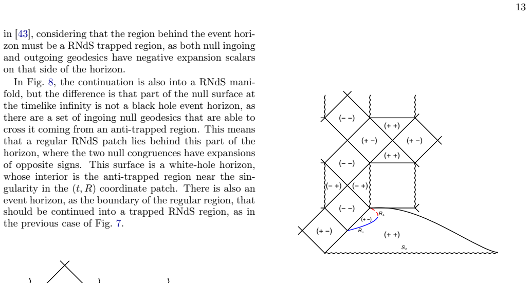
Analogously, if there existsδ >0 such that Fδ +(ti,t ) = ∫ t ti e(B+δ)u∆H(u) du, (71) converges ast→∞ , then a black-hole/white-hole pair is present

If there existsδ >0 such that Fδ −(ti,t ) = ∫ t ti e(B−δ)u∆H(u) du, (70) diverges ast→∞ , then a single black hole is present. Analogously, if there existsδ >0 such that Fδ +(ti,t ) = ∫ t ti e(B+δ)u∆H(u) du, (71) converges ast→∞ , then a black-hole/white-hole pair is present. ...
[14]

Region III In this case, Proposition IV.1 also applies to indicate what kind of region the ingoing null geodesics reach at the end of the coordinate patch near the ˆR− horizon. However, in this case ˆR− is not the innermost horizon, as we have yet another horizon, theˆR0 horiz...
[15]

In spacetimes represented by Region II there is no AH, and the patch covered by the coordinates is anti-trapped everywhere, therefore there is no doubt about the causal structure

Regions II and IV In these cases, the causal structure theorem and the Proposition IV.1 do not hold. In spacetimes represented by Region II there is no AH, and the patch covered by the coordinates is anti-trapped everywhere, therefore there is no doubt about the causal structu...
[16]

Following the reasoning of Sec

Application of the CST to a simple model Here we consider models with a Hubble function of the form H(t) =H0 coth (3H0t 2 ) , (72) where H0 is a positive constant. Following the reasoning of Sec. V of Ref. [14], we have the asymptotic form forFδ ±, Fδ ±∼ ∫ e(B−3H0±δ)u du. (73)...
[17]

2, represents an undercharged case with q < mand small mH0

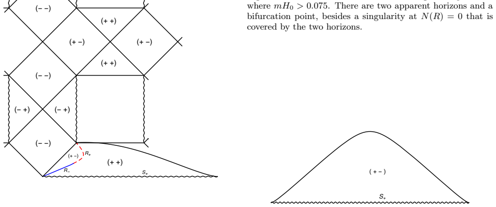
Region I This region, whose AHs and geodesic lines are pre- sented in Fig. 2, represents an undercharged case with q < mand small mH0. For such values of the param- eters there is a singularityS at R = m + √ m2−q2 that can be considered as an initial singularity, since it is s...
[18]

The singularity at R = m +√ m2−q2 is still present, however no AH is formed and the singularity is naked, as can be seen in Fig

Region II The solutions in this region correspond to asymp- totically undercharged RNdS spacetimes but now with higher values of mH0. The singularity at R = m +√ m2−q2 is still present, however no AH is formed and the singularity is naked, as can be seen in Fig. 3 and in the c...
[19]

They present three AHs, a singularity at 14 R = 0 and an initial singularity att = 0, as shown in Fig

Region III The solutions in this region correspond to spacetimes that asymptote to overcharged RNdS solution with1 < q/m <1.125. They present three AHs, a singularity at 14 R = 0 and an initial singularity att = 0, as shown in Fig. 4. These cases do not present a Cauchy surfac...
[20]

The Cauchy surface is not present either, as it can be seen in Fig

Region IV Finally, the fourth region contains overcharged SV spacetimes which also have a singularity atR = 0 and an initial singularity att = 0. The Cauchy surface is not present either, as it can be seen in Fig. 5. These solu- tions present one cosmological horizon (R−) that...

2014
[21]

A. M. was partially supported by CNPq Grant No. 400342/2017-0. This study was ﬁnanced in part by CAPES Finance Code 001. Appendix A: Regions of the parameter space In this Appendix, we study the cases in which the hori- zons are multiple roots ofP (x) deﬁned in Eq. (47), P (x)...

2017
[22]

This case correspondstotheverticalaxisinFig.1, andtheSVmet- ric (37) asymptotes to the Reissner–Nordström metric at large times

Singularities and horizons Assuming that the scale factor is a power law func- tion of the forma(t) = a0 +a1tα, withα >0, it follows that limt→∞H(t) = 0 and limt→∞ ˙H(t) = 0. This case correspondstotheverticalaxisinFig.1, andtheSVmet- ric (37) asymptotes to the Reissner–Nordst...
[23]

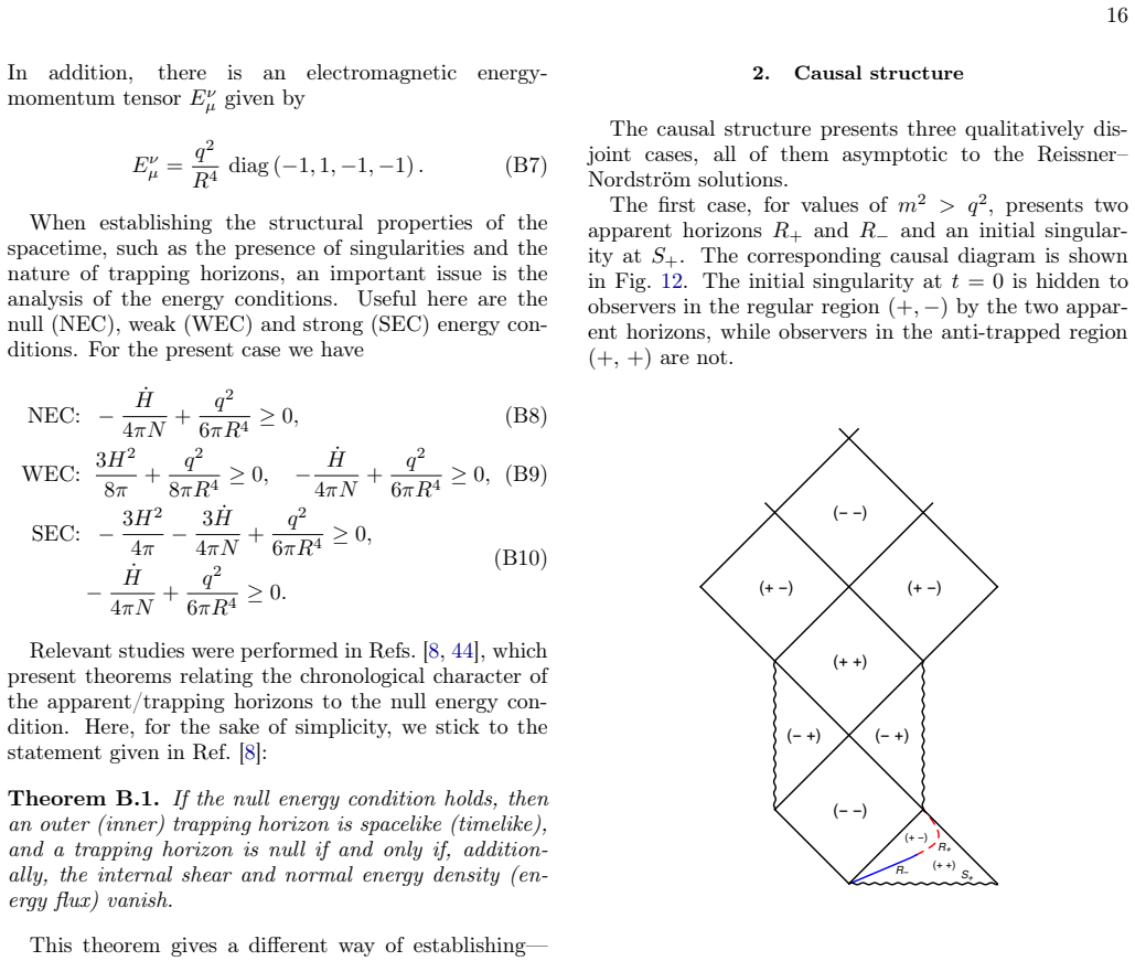
The ﬁrst case, for values ofm2 > q2, presents two apparent horizons R+ and R− and an initial singular- ity atS+

Causal structure The causal structure presents three qualitatively dis- joint cases, all of them asymptotic to the Reissner– Nordström solutions. The ﬁrst case, for values ofm2 > q2, presents two apparent horizons R+ and R− and an initial singular- ity atS+. The corresponding ...
[24]

B. P. Abbott et al. (LIGO Scientiﬁc Collaboration and Virgo Collaboration), Phys. Rev. Lett. 116, 241103 (2016), arXiv:1606.04855 [gr-qc]; Phys. Rev. Lett.116, 061102 (2016), arXiv:1602.03837 [gr-qc]

2016 arXiv
[25]

Akiyamaet al

K. Akiyamaet al. (Event Horizon Telescope), Astrophys. J. 875, L6 (2019); Astrophys. J.875, L2 (2019); Astro- phys. J.875, L3 (2019); Astrophys. J.875, L4 (2019); Astrophys. J.875, L5 (2019)

2019
[26]

Carlip, Int

S. Carlip, Int. J. Mod. Phys. D23, 1430023 (2014); J. D. Bekenstein, Phys. Rev. D7, 949 (1973); J. D. Beken- stein and M. Schiﬀer, Phys. Rev. D58, 064014 (1998); R. Brito, V. Cardoso, and P. Pani, Lect. Notes Phys. 906, 1 (2015), arXiv:1501.06570 [gr-qc]; S. W. Hawking, Commun...

2014 arXiv
[27]

S. N. G. Thakurta, Indian J. Phys. B55, 304 (1981); J. D. Barrow, E. J. Copeland, and A. R. Liddle, Mon. Not. R. Astron. Soc. 253, 675 (1991); J. Sultana and C. C. Dyer, Gen. Relativ. Gravit.37, 1347 (2005)

1981
[28]

M. L. McClure and C. C. Dyer, Class. Quantum Grav. 23, 1971 (2006)

2006
[29]

Faraoni, Galaxies1, 114 (2013), arXiv:1309.4915 [gr- qc]

V. Faraoni, Galaxies1, 114 (2013), arXiv:1309.4915 [gr- qc]

2013 arXiv
[30]

G. C. McVittie, Mon. Not. R. Astron. Soc. 92, 500 (1932); Mon. Not. R. Astron. Soc.93, 325 (1933)

1932
[31]

S. A. Hayward, Phys. Rev. D49, 831 (1994), arXiv:gr- qc/9303030 [gr-qc]; Phys. Rev. D 49, 6467 (1994), arXiv:gr-qc/9303006; Phys. Rev. D 53, 1938 (1996), arXiv:gr-qc/9408002 [gr-qc]; Class. Quantum Grav.15, 3147 (1998), arXiv:gr-qc/9710089 [gr-qc]

1994
[32]

J. M. Senovilla, Int. J. Mod. Phys. D20, 2139 (2011), arXiv:1107.1344 [gr-qc]; M. Mars and J. M. Sen- ovilla, Class. Quantum Grav.20, L293 (2003), arXiv:gr- qc/0309055 [gr-qc]

2011 arXiv
[33]

B. C. Nolan, Phys. Rev. D58, 064006 (1998), arXiv:gr- qc/9805041; Class. Quantum Grav. 16, 1227 (1999); Class. Quantum Grav. 16, 3183 (1999), arXiv:gr- qc/9907018; Class. Quantum Grav. 31, 235008 (2014), arXiv:1408.0044 [gr-qc]

1998
[34]

Carrera and D

M. Carrera and D. Giulini, Phys. Rev. D 81, 043521 (2010), arXiv:0908.3101 [gr-qc]

2010 arXiv
[35]

Kaloper, M

N. Kaloper, M. Kleban, and D. Martin, Phys. Rev. D 81, 104044 (2010), arXiv:1003.4777 [hep-th]

2010 arXiv
[36]

Lake and M

K. Lake and M. Abdelqader, Phys. Rev. D84, 044045 (2011), arXiv:1106.3666 [gr-qc]; M. Anderson, Journal of Physics: Conference Series283, 012001 (2011)

2011 arXiv
[37]

daSilva, M

A.M. daSilva, M. Fontanini, andD. C.Guariento,Phys. Rev. D87, 064030 (2013), arXiv:1212.0155 [gr-qc]

2013 arXiv
[38]

Landry, M

P. Landry, M. Abdelqader, and K. Lake, Phys. Rev. D 86, 084002 (2012), arXiv:1207.6350 [gr-qc]

2012 arXiv
[39]

Faraoni, A

V. Faraoni, A. F. Zambrano Moreno, and R. Nandra, Phys. Rev. D85, 083526 (2012), arXiv:1202.0719 [gr-qc]

2012 arXiv
[40]

19,191(1968)

Y.P.ShahandP.C.Vaidya,Tensor, N.S. 19,191(1968)

1968
[41]

Kastor and J

D. Kastor and J. Traschen, Phys. Rev. D47, 5370 (1993)

1993
[42]

J. B. Hartle and S. W. Hawking, Commun. Math. Phys. 26, 87 (1972)

1972
[43]

Nakao, T

K.-I. Nakao, T. Shiromizu, and S. A. Hayward, Phys. Rev. D52, 796 (1995)

1995
[44]

Chimento and D

S. Chimento and D. Klemm, J. High Energy Phys.2013, 129 (2013)

2013
[45]

Benone, E

J.-Z.Tang, (2009),arXiv:arXiv:0911.3849[hep-th]; C.L. Benone, E. S. de Oliveira, S. R. Dolan, and L. C. B. Crispino, (2014), arXiv:1404.0687 [gr-qc]

2009 arXiv
[46]

V.Faraoni, A.F.ZambranoMoreno, andA.Prain,Phys. Rev. D89, 103514 (2014), arXiv:1404.3929 [gr-qc]

2014 arXiv
[47]

M. G. Rodrigues and V. T. Zanchin, Class. Quantum Grav. 32, 115004 (2015), arXiv:1502.00688 [gr-qc]

2015 arXiv
[48]

R. Bibi, T. Clifton, and J. Durk, Gen. Rel. Grav.49, 98 (2017), arXiv:1705.01892 [gr-qc]

2017 arXiv
[49]

Afshordi, D

N. Afshordi, D. J. H. Chung, and G. Geshnizjani, Phys. Rev. D75, 083513 (2007), arXiv:hep-th/0609150; N. Af- shordi, D. J. H. Chung, M. Doran, and G. Geshnizjani, Phys.Rev.D 75,123509(2007),arXiv:astro-ph/0702002

2007 arXiv
[50]

R. A. Sussman, J. Math. Phys.28, 1118 (1987); J. Math. Phys.29, pp.945 (1988); J. Math. Phys.29, 1177 (1988)

1987
[51]

C. J. Gao and S. N. Zhang, Phys. Lett. B595, 28 (2004), arXiv:gr-qc/0407045 [gr-qc]

2004 arXiv
[52]

Abdalla, N

E. Abdalla, N. Afshordi, M. Fontanini, D. C. Guari- ento, and E. Papantonopoulos, Phys. Rev. D89, 104018 (2014), arXiv:1312.3682 [gr-qc]

2014 arXiv
[53]

Gomes and D

H. Gomes and D. C. Guariento, Phys. Rev. D95, 104049 (2017), arXiv:1703.08226 [gr-qc]

2017 arXiv
[54]

G. C. McVittie, Ann. Inst. Henri Poincaré Sec. A40, 235 (1984)

1984
[55]

Carrera and D

M. Carrera and D. Giulini, Rev. Mod. Phys. 82, 169 (2010)

2010
[56]

Faraoni, Symmetry7, 2038 (2015), arXiv:1510.03789 [gr-qc]

V. Faraoni, Symmetry7, 2038 (2015), arXiv:1510.03789 [gr-qc]

2015 arXiv
[57]

D. C. Guariento and F. Mercati, Phys. Rev. D94, 064023 (2016), arXiv:1606.01215 [gr-qc]

2016 arXiv
[58]

Dafermos, Class

M. Dafermos, Class. Quantum Grav. 22, 2221 (2005), arXiv:gr-qc/0403032 [gr-qc]

2005 arXiv
[59]

Schnetter and B

E. Schnetter and B. Krishnan, Phys. Rev. D73, 021502 (2006)

2006
[60]

Maciel, M

A. Maciel, M. Le Delliou, and J. P. Mimoso, Phys. Rev. D D92, 083525 (2015), arXiv:1506.07122 [gr-qc]

2015 arXiv
[61]

Maciel, Phys

A. Maciel, Phys. Rev. D 93, 104013 (2016), arXiv:1511.08663 [gr-qc]

2016 arXiv
[62]

Faraoni, (2015), arXiv:1508.06849 [gr-qc]

V. Faraoni, (2015), arXiv:1508.06849 [gr-qc]

2015 arXiv
[63]

Maciel, M

A. Maciel, M. Le Delliou, and J. P. Mimoso, Phys. Rev. D98, 024016 (2018), arXiv:1803.11547 [gr-qc]

2018 arXiv
[64]

A. M. da Silva, D. C. Guariento, and C. Molina, Phys. Rev. D91, 084043 (2015), arXiv:1502.01003 [gr-qc]

2015 arXiv
[65]

Walker, J

M. Walker, J. Math. Phys.11, 2280 (1970)

1970
[66]

Laue and M

H. Laue and M. Weiss, Phys. Rev. D16, 3376 (1977)

1977
[67]

Andersson, M

L. Andersson, M. Mars, and W. Simon, Phys. Rev. Lett. 95, 111102 (2005), arXiv:gr-qc/0506013 [gr-qc]

2005 arXiv

Pith tools

Reviewed August 14, 2026 · model on record in the stance chip above.

[1] [1]

(14), we ﬁnd the same solution for the potential as in [29],i.e., (dV dφ )2 = 3µ4V , (34) V = 3µ4 4 (φ−V0)2 , (35) and it is then seen that the entire system is consistent

Combining this relation with the equation of motion of the cuscuton ﬁeld, Eq. (14), we ﬁnd the same solution for the potential as in [29],i.e., (dV dφ )2 = 3µ4V , (34) V = 3µ4 4 (φ−V0)2 , (35) and it is then seen that the entire system is consistent. In summary, we have shown that the Shah–Vaidya metric is an exact solution of the Einstein–Maxwell equatio...

work page

[2] [2]

Hence, considering that the isotropic coordinate is real, the domain of the areal radius coordi- nateR should be restricted to the intervalsR+≤R< ∞ and 0≤R≤R−

Undercharged case: m2 >q 2 In this case, the lapse function N(R) has two roots R± =m± √ m2−q2, andN 2(R) is negative in the inter- valR− <R<R +. Hence, considering that the isotropic coordinate is real, the domain of the areal radius coordi- nateR should be restricted to the intervalsR+≤R< ∞ and 0≤R≤R−. If one assumes, as usual, that the areal radius rang...

work page

[3] [3]

We then conclude that, form2 =q2, theisotropiccoordinate r covers(once) all the range ofR

Extremal case: m2 =q2 In this case, N(R) has a double root R+ = R− = m =|q|, andN 2(R) is non-negative in the whole domain 0≤R< ∞, where it is assumed, as usual, that the areal radius ranges from zero to inﬁnity. We then conclude that, form2 =q2, theisotropiccoordinate r covers(once) all the range ofR. Equation (36) reduces toR =ar +m, and so the region R...

work page

[4] [4]

Therefore, form2 <q 2, the isotropic coordinate r covers (twice) all the range ofR

Overcharged case: m2 <q 2 Inthiscase, N(R)hasnorealrootsand N 2(R)remains nonzero in the whole domain0≤R< ∞, where it is as- sumed, as usual, that the areal radius ranges from zero to inﬁnity. Therefore, form2 <q 2, the isotropic coordinate r covers (twice) all the range ofR. Indeed, the full range R∈ [0,∞) is covered once byar∈ [(−m +|q|)/2,∞), and again...

work page

[5] [5]

(36) and (39)] for which the a(t)r→ 0 limit corresponds toR→∞ , whileR = 0 cor- responds to a(t)r = (−m±|q|)/2, where the isotropic coordinater is allowed to assume negative values

Undercharged case: m2 >q 2 Let us choose the positive branch of the isotropic ra- dial coordinate [see Eqs. (36) and (39)] for which the a(t)r→ 0 limit corresponds toR→∞ , whileR = 0 cor- responds to a(t)r = (−m±|q|)/2, where the isotropic coordinater is allowed to assume negative values. Is this case, when m2 > q2, the function N(R) has two real positive...

work page

[6] [6]

First of all, Eq

Extremely charged case m2 =q2 This is a particular but very interesting situation for these solutions. First of all, Eq. (36) becomes R = a(t)r +m, so that R = 0 corresponds to r =−m/a. The lapse function N(R) has only one positive root, R =R± =m, which corresponds to a singularity of the curvature scalars. The relevant spacetimes are obtained by choosing...

work page

[7] [7]

The spacetime de- scribed by the overcharged SV metric includes all the range of the radial coordinate0<R< ∞and is bounded by a singular timelike surface atR = 0

Overcharged case: m2 <q 2 In this case, the lapse function has no roots and there is a curvature singularity atR = 0. The spacetime de- scribed by the overcharged SV metric includes all the range of the radial coordinate0<R< ∞and is bounded by a singular timelike surface atR = 0. Similarly to the static overcharged Reissner– Nordström–de Sitter (RNdS) cas...

work page

[8] [8]

Regions I and II Regions I and II cover the whole region of the param- eter space forσ2 < 1, and are separated by the curve for σ2 c−, the dashed line in Fig. 1. Region I is a bounded re- gion, while region II is unbounded, extending toh→∞ . In this case, we may have between one end three real roots for Eq. (47), but the smallest of them is always be- low...

work page