REVIEW 3 major objections 3 minor 52 references
Self-Boost via Optimal Retraining: An Analysis via Approximate Message Passing
T0 review · 3 major / 3 minor · reviewed 2026-08-07 · deepseek-v4-flash
Pith's one-line read For binary classification with noisy labels, the paper derives the Bayes-optimal rule for combining a model's predictions with the given labels, and shows it minimizes prediction error across retraining rounds.
desk verdict A clean optimal-aggregator derivation with a real factor-α error in the stated state evolution; worth refereeing after a careful revision. read the letter →
The pith
A machine-rendered reading of the paper's core claim, the machinery that carries it, and where it could break.
The reading
What carries the argument
The machinery is the AMP update (4)-(5), whose Onsager correction terms debias the iterates so their empirical distributions become asymptotically Gaussian, and the companion state-evolution recursion (7) that tracks the means and variances $(m_t, \sigma_t)$. The decisive object is the posterior probability $q_t = P(Y=1 \mid \bar{m}_t Y + \bar{\sigma}_t G, \hat{Y})$; a Cauchy-Schwarz argument shows that any aggregator's signal-to-noise ratio $m_{t+1}/\sigma_{t+1}$ is bounded by $E[(2q_t-1)^2]$, and this bound is attained exactly by the Bayes-optimal rule $g_t^* = 2q_t-1$. The formulas (13) and (25) are the explicit Bayes-rule evaluations of that posterior mean in the two data models, and the recursions (14) and (26) reduce the whole retraining trajectory to the evolution of the single ratio $\eta_t = m_t/\sigma_t$.
What would settle it
Run the AMP updates (4)-(5) on finite-$n$ GMM data with the claimed optimal aggregator and compare the realized test error to the predicted $\Phi(-\gamma\eta_t/\sqrt{\eta_t^2+1})$ for a sequence of growing $n$ and fixed $t$: a persistent gap, or a failure of the empirical distribution of entries of $\theta_t$ to match a Gaussian with variance $m_t^2+\sigma_t^2$, would show the state-evolution premise fails. A second check is to search numerically over aggregators for one that beats $g_t^*$ in the $m_{t+1}/\sigma_{t+1}$ ratio at any round, which would contradict Theorem 3.2 directly.
Extended reading notes
Core claim
The central claim is that the optimal aggregator at round $t$ is the posterior-mean rule $g_t^*(y,\hat{y}) = 2/(1+(p/(1-p))^{\hat{y}} \exp(-2\gamma^2 y/(\alpha(\eta_t^2+1))) \pi_-/\pi_+) - 1$ for the GMM, with an analogous integral-based formula for GLMs (Theorems 3.2 and 4.3). This choice is optimal in the sense of maximizing the ratio $m_{t+1}/\sigma_{t+1}$ that controls the next model's test error; because the state-evolution map is non-decreasing in the GMM case, the aggregator also minimizes the classification error at every subsequent round. The paper further shows that retraining with this rule can be characterized by a one-dimensional recursion $\eta_{t+1}^2 = F(\eta_t^2)$, so the effect of many rounds is deterministic and quantifiable.
Load-bearing premise
The load-bearing premise is that AMP state evolution correctly describes the empirical distribution of the estimates for the paper's recursions with data-dependent initialization, a result quoted from standard AMP/GAMP theory (with the GMM proof omitted) rather than proved here.
Editorial extensions
If this is right
- With the optimal aggregator, each retraining round is guaranteed (in the asymptotic limit) not to decrease the signal-to-noise ratio when starting below the fixed point, and the one-dimensional map $F$ predicts exactly how test error improves over rounds.
- If the initial model is poor ($\eta_1$ below the fixed point), retraining strictly reduces test error; if the initial model is already very good, Proposition 3.3 shows retraining can actually hurt, matching the paper's observation that the fixed point is a separator.
- In the GMM setting, the Bayes-optimal choice at a single round also minimizes test error at all future rounds because $F$ is non-decreasing, so there is no trade-off between short-term and long-term gains.
- The practical BayesMix RT rule, which fits a bimodal GMM to logits and applies a similarly derived aggregator, improves on full retraining and consensus-based retraining by a large margin on Food-101 Pho-vs-Ramen at label-flip probability $p=0.45$ after 10 rounds.
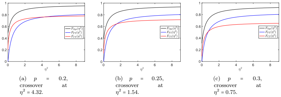
- Synthetic experiments in the paper show the AMP theory with the optimal aggregator tracks simulation closely, and the optimal map dominates the full-retraining and consensus maps at every $\eta$ in the examples.
Reading between the lines
- The optimal aggregator has a readable shrinkage form: it down-weights the noisy label by a factor depending on the model's soft prediction, effectively treating the model output as an extra noisy observation of the true label; the same principle could be ported to nonlinear models by estimating the needed moments from logits.
- Because AMP is conjectured optimal among polynomial-time algorithms for many high-dimensional estimation problems, the paper's framework suggests the Bayes-optimal retraining rule may also be computationally optimal for these data models, a claim the paper does not itself make.
- A direct testable extension is to estimate the label-flip probability $p$ online and re-fit the bimodal GMM each round; the state-evolution map predicts the gap between BayesMix RT and consensus-based retraining should widen as $p$ approaches $1/2$ and shrink as $p$ decreases, which Table 5 qualitatively supports.
Editorial analysis
A structured set of objections, weighed in public.
Referee Report
Summary. The paper studies iterative retraining of a binary classifier when the observed labels are noisy. It proposes an AMP-style iterative update in which, at each round, the current soft predictions and the noisy labels are combined by an aggregator function, and it derives the Bayes-optimal aggregator for two data models: a Gaussian mixture model (GMM) and a generalized linear model (GLM). For the GMM it gives a state-evolution recursion, a closed-form optimal aggregator, and a monotonicity result showing when retraining helps or hurts; for the GLM it gives an analogous state-evolution characterization and an optimal aggregator expressed through an integral. The paper also proposes a practical variant, BayesMix RT, obtained by fitting a bimodal Gaussian to the logits of a pretrained model, and reports experiments on two image classification tasks in the high-label-noise regime.
Significance. If the state-evolution theorems are correct, the paper provides a principled and fairly complete answer to a question that previous retraining literature addressed only heuristically: how to optimally combine a model's own predictions with noisy labels during retraining. The derivation of the optimal aggregator as a Bayes posterior ratio is clean, checkable, and is a genuine conceptual contribution. The paper also ships synthetic simulations that verify the corrected state evolution, and the proposed BayesMix RT method is a natural, falsifiable practical extension. These strengths make the paper potentially valuable for the AMP and noisy-label retraining communities, provided the recursion inconsistencies described below are resolved.
major comments (3)
- [Section 3.2, Eq. (7); Section 3.3, Eqs. (10)-(12) and (14)] The state-evolution recursion is stated with an incorrect factor. Taking the admissible aggregator g_t(y, yhat) = yhat gives theta_{t+1} = theta_t and y_{t+1} = y_t, so the state evolution must satisfy m_{t+1} = m_1 = gamma (1-2p)/sqrt(alpha). Substituting g_t = yhat into Eq. (7) at t=1 gives m_2 = gamma sqrt(alpha) (1-2p), which differs by a factor alpha. The correct update is m_{t+1} = (gamma/sqrt(alpha)) E[Y g_t(barm_t Y + barsigma_t G, Yhat)], which is the form implicitly used by Eq. (10), Eq. (12), and Eq. (14). Eq. (11) repeats the gamma sqrt(alpha) error and contradicts Eq. (12), because Eq. (12) implies m_t = (gamma/sqrt(alpha)) sigma_t^2. As printed, Theorem 3.1 is false, and the optimal-aggregator claim in Theorem 3.2 depends on this recursion.
- [Appendix A (proof of Theorem 3.1) and Appendix G (Theorem 4.2)] The state-evolution theorems are not proved. Appendix A states that the proof 'follows by adapting techniques from standard AMP analysis ... and so omitted here', and Theorem 4.2 is delegated to the GAMP results of [36]. Because the updates (4)-(5) and (16)-(17) include memory corrections and a data-dependent initialization g_0(., yhat) = yhat, this is not a routine invocation unless a precise external theorem covers exactly this recursion and initialization. This is load-bearing: Theorem 3.2, Theorem 4.3, and the test-error formulas (9) and (23) all rest on these state-evolution results. Please provide a complete proof or a precise statement of the external theorem being applied, and re-check the initialization argument after the recursion factors are corrected.
- [Section 4, Theorem 4.2 vs. Appendix G] The GLM state evolution contains an analogous factor-alpha inconsistency. Theorem 4.2 as printed states the limiting empirical distribution of beta_t with sigma_t sqrt(alpha) multiplying the Gaussian variable, while the derivation in Appendix G computes E[(mu_t betabar + sigma_t/sqrt(alpha) G)^2] and uses the sigma_t/sqrt(alpha) form to obtain the expression eta_t gamma / sqrt(eta_t^2 gamma^2 + 1/alpha) in Eq. (23). These two displays differ by a factor alpha. As typeset, the GLM state-evolution theorem is internally inconsistent; please correct either the statement of Theorem 4.2 or the appendix computation and verify the initialization mu_1 = 2 E[Z hhat_p(Z)]/(alpha gamma^2), sigma_1 = sqrt(alpha) against the corrected recursion.
minor comments (3)
- [Section 5 and Appendix K] In the experiments, each method uses a different retraining learning rate (eta_1 = 5e-4, 1e-4, or 5e-6 across methods). Since the learning rate can strongly affect linear probing results, please include a matched-learning-rate comparison or an ablation over learning rates so the reported gains of BayesMix RT are not attributable to this difference.
- [Section 3.3, discussion after Eq. (15) and Proposition 3.3] The text says that 'if the initial model is already good, retraining can actually hurt its performance', but Proposition 3.3(i) only proves that the sequence is non-decreasing when eta_1 <= eta_*. It does not prove monotone decrease for eta_1 above the smallest fixed point. Please add a proof or qualify the claim.
- [Appendix K] The learning-rate symbols eta_0 and eta_1 in Appendix K conflict with the state-evolution variable eta_t used throughout the paper; consider renaming the learning rates to avoid confusion.
Circularity Check
No significant circularity: the optimal aggregator is derived from the assumed data model via Bayes rule and Cauchy-Schwarz, with AMP state evolution cited as standard external theory.
full rationale
The paper's central claim is a mathematical derivation, not a fitted prediction. Given the AMP state-evolution recursion, the optimal aggregator is obtained by maximizing m_{t+1}/sigma_{t+1}: Eq. (10) applies Cauchy-Schwarz and achievability identifies g_t^* as the conditional mean 2q_t-1; Theorem 3.2 then computes this posterior mean explicitly by Bayes rule. Nothing in this chain is defined in terms of its own output, and no parameter is fitted to the test quantity being predicted. The empirical BayesMix RT in Section 5 does fit a bimodal GMM to logits, but the paper explicitly disclaims that this practical variant is necessarily optimal on real data (footnote 4), so the claimed empirical superiority is an experimental comparison, not a circular prediction. The self-citations ([9] for baselines, [18] for AMP) are not load-bearing in a circular way: [18] is a standard external state-evolution result whose assumptions do not contain the target result, and [9] only defines the baseline retraining rules. The omitted proof of Theorem 3.1 is a support gap, and the printed Eq. (7) appears internally inconsistent with Eqs. (10)-(14) (a correctness concern), but neither is an equivalence-by-construction or a fitted-input-as-prediction, so they do not count as circularity.
Assumptions & free parameters
free parameters (2)
- Bimodal GMM parameters of logits (mu_+, sigma_+, mu_-, sigma_-, pi_+, pi_-) =
Fitted per dataset from training logits; no numbers reported
- Retraining learning rate eta_1 =
5e-4 for full RT and consensus RT, 5e-6 for BayesMix RT on Food-101; 5e-4 for all on MedMNIST
assumptions (5)
- standard math Validity of AMP state evolution for Gaussian random matrices and GAMP convergence (Bayati-Montanari 2011, Rangan 2011, Javanmard-Montanari 2013)
- domain assumption Asymptotic regime n,d go to infinity with d/n to alpha and weak convergence of empirical distributions of features and coefficients (Assumptions 1 and 2)
- domain assumption Uniform, independent label flipping with probability p < 1/2 (noise model (2))
- domain assumption Test error monotonicity: for GMM, P_e = Phi(-gamma eta / sqrt(eta^2+1)) decreases in eta; for GLM, F(rho) decreases when h(u) > h(-u) for u > 0 (Lemma 4.1)
- ad hoc to paper The logits of the pretrained model follow a bimodal Gaussian distribution in the practical BayesMix RT method
Cite this review
Pith. "Pith review of Self-Boost via Optimal Retraining: An Analysis via Approximate Message Passing." pith.science (2026). https://pith.science/paper/IO7JK7AQ
@misc{pith2026250515195,
  author       = {Pith},
  title        = {Pith review of: Self-Boost via Optimal Retraining: An Analysis via Approximate Message Passing},
  year         = {2026},
  howpublished = {\url{https://pith.science/paper/IO7JK7AQ}},
  note         = {Machine review of arXiv:2505.15195}
}
read the original abstract
Retraining a model using its own predictions together with the original, potentially noisy labels is a well-known strategy for improving the model performance. While prior works have demonstrated the benefits of specific heuristic retraining schemes, the question of how to optimally combine the model's predictions and the provided labels remains largely open. This paper addresses this fundamental question for binary classification tasks. We develop a principled framework based on approximate message passing (AMP) to analyze iterative retraining procedures for two ground truth settings: Gaussian mixture model (GMM) and generalized linear model (GLM). Our main contribution is the derivation of the Bayes optimal aggregator function to combine the current model's predictions and the given labels, which when used to retrain the same model, minimizes its prediction error. We also quantify the performance of this optimal retraining strategy over multiple rounds. We complement our theoretical results by proposing a practically usable version of the theoretically-optimal aggregator function for linear probing with the cross-entropy loss, and demonstrate its superiority over baseline methods in the high label noise regime.
Figures


Figures from the paper (3 more)


Reference graph
Works this paper leans on
-
[36]
In2011 IEEE International Symposium on Information Theory Proceedings(2011), IEEE, pp
Rangan, S.Generalized approximate message passing for estimation with random linear mixing. In2011 IEEE International Symposium on Information Theory Proceedings(2011), IEEE, pp. 2168–2172
work page 2011
-
[1]
Alain, G., and Bengio, Y.Understanding intermediate layers using linear classifier probes.arXiv preprint arXiv:1610.01644(2016)
arXiv 2016
-
[2]
Amini, M.-R., Feof anov, V., Pauletto, L., Devijver, E., and Maximov, Y.Self- training: A survey.arXiv preprint arXiv:2202.12040(2022)
arXiv 2022
-
[3]
Barbier, J., Krzakala, F., Macris, N., Miolane, L., and Zdeborová, L.Optimal errors and phase transitions in high-dimensional generalized linear models.Proceedings of the National Academy of Sciences 116, 12 (2019), 5451–5460
work page 2019
-
[4]
Bayati, M., and Montanari, A.The dynamics of message passing on dense graphs, with applications to compressed sensing.IEEE Transactions on Information Theory 57, 2 (2011), 764–785
work page 2011
-
[5]
Bayati, M., and Montanari, A.The lasso risk for gaussian matrices.IEEE Transactions on Information Theory 58, 4 (2011), 1997–2017. 11
work page 2011
-
[6]
InEuropean Conference on Computer Vision(2014)
Bossard, L., Guillaumin, M., and V an Gool, L.Food-101 – mining discriminative components with random forests. InEuropean Conference on Computer Vision(2014)
work page 2014
-
[7]
Carmon, Y., Raghunathan, A., Schmidt, L., Duchi, J. C., and Liang, P. S. Unlabeled data improves adversarial robustness.Advances in neural information processing systems 32(2019)
work page 2019
Show all 52 references
-
[8]
Chen, Y., Wei, C., Kumar, A., and Ma, T.Self-training avoids using spurious features under domain shift.Advances in Neural Information Processing Systems 33(2020), 21061–21071
2020
-
[9]
Das, R., Dhillon, I. S., Epasto, A., Ja v anmard, A., Mao, J., Mirrokni, V., Sangha vi, S., and Zhong, P.Retraining with predicted hard labels provably increases model accuracy.arXiv preprint arXiv:2406.11206(2024)
2024 arXiv
-
[10]
InInternational Conference on Machine Learning(2023), PMLR, pp
Das, R., and Sangha vi, S.Understanding self-distillation in the presence of label noise. InInternational Conference on Machine Learning(2023), PMLR, pp. 7102–7140
2023
-
[11]
arXiv preprint arXiv:1910.01255(2019)
Dong, B., Hou, J., Lu, Y., and Zhang, Z.Distillation ≈ early stopping? harvesting dark knowledge utilizing anisotropic information retrieval for overparameterized neural network. arXiv preprint arXiv:1910.01255(2019)
2019 arXiv
-
[12]
Donoho, D. L., Ja v anmard, A., and Montanari, A.Information-theoretically optimal compressed sensing via spatial coupling and approximate message passing.IEEE transactions on information theory 59, 11 (2013), 7434–7464
2013
-
[13]
L., Maleki, A., and Montanari, A.Message-passing algorithms for compressed sensing.Proceedings of the National Academy of Sciences 106, 45 (2009), 18914–18919
Donoho, D. L., Maleki, A., and Montanari, A.Message-passing algorithms for compressed sensing.Proceedings of the National Academy of Sciences 106, 45 (2009), 18914–18919
2009
-
[14]
Y., Venkataramanan, R., Rush, C., Samworth, R
Feng, O. Y., Venkataramanan, R., Rush, C., Samworth, R. J., et al.A unifying tutorial on approximate message passing.Foundations and Trends®in Machine Learning 15, 4 (2022), 335–536
2022
-
[15]
InInternational Conference on Machine Learning(2018), PMLR, pp
Furlanello, T., Lipton, Z., Tschannen, M., Itti, L., and Anandkumar, A.Born again neural networks. InInternational Conference on Machine Learning(2018), PMLR, pp. 1607–1616
2018
-
[16]
Goel, A., Jiao, Y., and Massiah, J.Pars: Pseudo-label aware robust sample selection for learning with noisy labels.arXiv preprint arXiv:2201.10836(2022)
2022 arXiv
-
[17]
InProceedings of the IEEE/CVF international conference on computer vision(2019), pp
Han, J., Luo, P., and W ang, X.Deep self-learning from noisy labels. InProceedings of the IEEE/CVF international conference on computer vision(2019), pp. 5138–5147
2019
-
[18]
Ja v anmard, A., and Montanari, A.State evolution for general approximate message passing algorithms, with applications to spatial coupling.Information and Inference: A Journal of the IMA 2, 2 (2013), 115–144
2013
-
[19]
Kabashima, Y., Krzakala, F., Mézard, M., Sakata, A., and Zdeborová, L.Phase transitions and sample complexity in bayes-optimal matrix factorization.IEEE Transactions on information theory 62, 7 (2016), 4228–4265
2016
-
[20]
1: Distribution theory.London [etc.]: Arnold [etc.](1994)
Kendall, M., Stuart, A., and Ord, J.Vol. 1: Distribution theory.London [etc.]: Arnold [etc.](1994)
1994
-
[21]
InInternational conference on machine learning(2020), PMLR, pp
Kumar, A., Ma, T., and Liang, P.Understanding self-training for gradual domain adaptation. InInternational conference on machine learning(2020), PMLR, pp. 5468–5479. 12
2020
-
[22]
Kumar, A., Raghunathan, A., Jones, R., Ma, T., and Liang, P.Fine-tuning can distort pretrained features and underperform out-of-distribution.arXiv preprint arXiv:2202.10054(2022)
2022 arXiv
-
[23]
InWorkshop on challenges in representation learning, ICML (2013), vol
Lee, D.-H., et al.Pseudo-label: The simple and efficient semi-supervised learning method for deep neural networks. InWorkshop on challenges in representation learning, ICML (2013), vol. 3, Atlanta, p. 896
2013
-
[24]
C.Dividemix: Learning with noisy labels as semi- supervised learning.arXiv preprint arXiv:2002.07394(2020)
Li, J., Socher, R., and Hoi, S. C.Dividemix: Learning with noisy labels as semi- supervised learning.arXiv preprint arXiv:2002.07394(2020)
2020 arXiv
-
[25]
InProceedings of the IEEE International Conference on Computer Vision (2017), pp
Li, Y., Yang, J., Song, Y., Cao, L., Luo, J., and Li, L.-J.Learning from noisy labels with distillation. InProceedings of the IEEE International Conference on Computer Vision (2017), pp. 1910–1918
2017
-
[26]
Mobahi, H., F arajtabar, M., and Bartlett, P.Self-distillation amplifies regularization in hilbert space.Advances in Neural Information Processing Systems 33(2020), 3351–3361
2020
-
[27]
InInternational Conference on Artificial Intelligence and Statistics(2021), PMLR, pp
Mondelli, M., and Venkataramanan, R.Approximate message passing with spec- tral initialization for generalized linear models. InInternational Conference on Artificial Intelligence and Statistics(2021), PMLR, pp. 397–405
2021
-
[28]
Montanari, A., Eldar, Y., and Kutyniok, G.Graphical models concepts in compressed sensing.Compressed Sensing(2012), 394–438
2012
-
[29]
Montanari, A., and Richard, E.Non-negative principal component analysis: Message passing algorithms and sharp asymptotics.IEEE Transactions on Information Theory 62, 3 (2015), 1458–1484
2015
-
[30]
Montanari, A., and Venkataramanan, R.Estimation of low-rank matrices via approximate message passing.The Annals of Statistics 49, 1 (2021)
2021
-
[31]
T., Mummadi, C
Nguyen, D. T., Mummadi, C. K., Ngo, T. P. N., Nguyen, T. H. P., Beggel, L., and Brox, T.Self: Learning to filter noisy labels with self-ensembling.arXiv preprint arXiv:1910.01842(2019)
2019 arXiv
-
[32]
C.Statistical and algorithmic insights for semi-supervised learning with self-training.arXiv preprint arXiv:2006.11006(2020)
Oymak, S., and Gulcu, T. C.Statistical and algorithmic insights for semi-supervised learning with self-training.arXiv preprint arXiv:2006.11006(2020)
2020 arXiv
-
[33]
S., and Oh, S.Understanding the gains from repeated self-distillation
Pareek, D., Du, S. S., and Oh, S.Understanding the gains from repeated self-distillation. arXiv preprint arXiv:2407.04600(2024)
2024 arXiv
-
[34]
S., Bandeira, A
Perry, A., Wein, A. S., Bandeira, A. S., and Moitra, A.Message-passing algorithms for synchronization problems over compact groups.Communications on Pure and Applied Mathematics 71, 11 (2018), 2275–2322
2018
-
[35]
M., Yang, F., Duchi, J., and Liang, P.Understanding and mitigating the tradeoff between robustness and accuracy.arXiv preprint arXiv:2002.10716 (2020)
Raghunathan, A., Xie, S. M., Yang, F., Duchi, J., and Liang, P.Understanding and mitigating the tradeoff between robustness and accuracy.arXiv preprint arXiv:2002.10716 (2020)
2020 arXiv
-
[37]
K.Iterative estimation of constrained rank-one matrices in noise
Rangan, S., and Fletcher, A. K.Iterative estimation of constrained rank-one matrices in noise. In2012 IEEE international symposium on information theory proceedings(2012), IEEE, pp. 1246–1250. 13
2012
-
[38]
Reed, S., Lee, H., Anguelov, D., Szegedy, C., Erhan, D., and Rabinovich, A.Training deep neural networks on noisy labels with bootstrapping.arXiv preprint arXiv:1412.6596(2014)
2014 arXiv
-
[39]
Scudder, H.Probability of error of some adaptive pattern-recognition machines.IEEE Transactions on Information Theory 11, 3 (1965), 363–371
1965
-
[40]
Takanami, K., Takahashi, T., and Sakata, A.The effect of optimal self-distillation in noisy gaussian mixture model.arXiv preprint arXiv:2501.16226(2025)
2025
-
[41]
InProceedings of the IEEE conference on computer vision and pattern recognition(2018), pp
Tanaka, D., Ikami, D., Yamasaki, T., and Aiza w a, K.Joint optimization framework for learning with noisy labels. InProceedings of the IEEE conference on computer vision and pattern recognition(2018), pp. 5552–5560
2018
-
[42]
Wei, C., Shen, K., Chen, Y., and Ma, T.Theoretical analysis of self-training with deep networks on unlabeled data.arXiv preprint arXiv:2010.03622(2020)
2020 arXiv
-
[43]
Yang, J., Shi, R., Wei, D., Liu, Z., Zhao, L., Ke, B., Pfister, H., and Ni, B.Medmnist v2-a large-scale lightweight benchmark for 2d and 3d biomedical image classification.Scientific Data 10, 1 (2023), 41
2023
-
[44]
In 33rd annual meeting of the association for computational linguistics(1995), pp
Yarowsky, D.Unsupervised word sense disambiguation rivaling supervised methods. In 33rd annual meeting of the association for computational linguistics(1995), pp. 189–196
1995
-
[45]
Zhang, S., W ang, M., Liu, S., Chen, P.-Y., and Xiong, J.How does unlabeled data improve generalization in self-training? a one-hidden-layer theoretical analysis.arXiv preprint arXiv:2201.08514(2022). 14 Appendix A Proof of Theorem 3.1 To build some intuition on the statement ...
2022 arXiv
-
[46]
Hence, the first step strictly reduces the test error and the next rounds of retraining do not increase the test error
Further, by monotonicity of F, per item (i), ifη2 t ≤η 2 t+1, then η2 t+1 =F(η 2 t)≤F(η 2 t+1)=η 2 t+2, which proves that the sequence(ηt)t≥1 is monotone non-decreasing. Hence, the first step strictly reduces the test error and the next rounds of retraining do not increase the...
-
[47]
To this end, we derive a lower bound onF, such that ˜F(u)<F(u) , ∀u≥ 0, and establish condition on the label flipping probabilityp, so that η2 1 ≤ ˜F(η 2
then the sequence(ηt)t≥1 will be non-decreasing. To this end, we derive a lower bound onF, such that ˜F(u)<F(u) , ∀u≥ 0, and establish condition on the label flipping probabilityp, so that η2 1 ≤ ˜F(η 2
-
[48]
17 To construct ˜F, recall that˜gis the Bayes-optimal aggregator given by˜g(˜Y ,̂Y)=E[Y∣ ˜Y= ¯ηY+√¯ηG,̂Y]
with η1 = γ√α(1−2p). 17 To construct ˜F, recall that˜gis the Bayes-optimal aggregator given by˜g(˜Y ,̂Y)=E[Y∣ ˜Y= ¯ηY+√¯ηG,̂Y]. Using the Cauchy–Schwarz inequality for allg, E[˜g(˜Y ,̂Y) 2]≥ E[E[Y∣ ˜Y ,̂Y]g( ˜Y ,̂Y)] 2 E[g( ˜Y ,̂Y) 2] = E[Y g(˜Y ,̂Y)] 2 E[g( ˜Y ,̂Y) 2] with ˜g...
-
[49]
These properties give a clear picture of the function h: it will be positive on[0, p∗), negative on(p∗, 1
Also note thath is a convex function becauseh′′(p)> 0, and therefore, these are the only two zeros ofh. These properties give a clear picture of the function h: it will be positive on[0, p∗), negative on(p∗, 1
-
[50]
Hence, condition(32), i.e.,h(p)≤0holds ifp∈[p ∗, 1 2), which completes the proof
and positive afterward. Hence, condition(32), i.e.,h(p)≤0holds ifp∈[p ∗, 1 2), which completes the proof. D Simulations to Verify the Theory in Section 3 In Figure 2, we compare the performance of different retraining methods on synthetic data, generated from a GMM model. The ...
-
[51]
The test set consists of 624 examples
MedMNISTPneumonia( https://www.tensorflow.org/datasets/catalog/pneumonia_ mnist): This has 4708 training examples and comes with a validation set of size 200. The test set consists of 624 examples. Here,η0 =5e−5andη 1 =5e−4for all three methods
-
[52]
Ramen( https://www.tensorflow.org/datasets/catalog/food101): Each class in Food-101 has 750 training examples; so the total number of examples for the two classes is 1500
Food-101: Phovs. Ramen( https://www.tensorflow.org/datasets/catalog/food101): Each class in Food-101 has 750 training examples; so the total number of examples for the two classes is 1500. Out of these 1500 examples, we randomly select 100 examples as our validation set. The t...
Reviewed August 7, 2026 · model on record in the stance chip above.
Discussion (0). Sign in to comment.