REVIEW 3 major objections 5 minor 41 references
Policy Newton Algorithm in Reproducing Kernel Hilbert Space
T0 review · 3 major / 5 minor · reviewed 2026-08-07 · deepseek-v4-flash
Pith's one-line read The paper claims that RL policies in a reproducing kernel Hilbert space can be trained with a second-order Newton step obtained from a cubic-regularized auxiliary objective, and that this step reduces to a finite-dimensional coefficient…
desk verdict The big idea is promising, but Theorem 3.3 swaps the RKHS norm for a Euclidean norm, so the algorithm analyzed is not the algorithm implemented. read the letter →
The pith
A machine-rendered reading of the paper's core claim, the machinery that carries it, and where it could break.
The reading
What carries the argument
The load-bearing object is the cubic-regularized auxiliary objective in the RKHS: it packages the gradient, the Hessian operator, and a cubic penalty $\tfrac{\beta}{6}\|\bar h\|^3$ into a single optimization whose minimizer is the update step. The Hessian enters as an operator on $H_K\otimes H_K$ built from outer products of kernel sections and per-state covariance operators, so its action on any candidate update is computable even though the operator itself cannot be inverted in closed form. The Representer Theorem then converts the search over functions $h\in H_K$ into a search over a coefficient vector $\bar\alpha\in\mathbb{R}^{NT}$, and Theorem 3.3 records the precise coefficient vector $v$ and matrix $H$ for the first- and second-order terms. The cubic penalty is what makes the subproblem strongly regularized, enabling the stationary-point and quadratic-convergence arguments.
What would settle it
Take any fixed batch of state-action points and a kernel whose Gram matrix has nonzero off-diagonal entries, and evaluate $\tfrac{\beta}{6}\|\sum_i \alpha_i K(x_i,\cdot)\|_{H_K}^3$ alongside $\tfrac{\beta}{6}\|\alpha\|_2^3$ at one shared $\alpha$: if the values differ, Equation (7) is not equivalent to Equation (5). A reader could then check whether the local quadratic error bound of Theorem 4.6 still holds when the update is computed from the true RKHS cubic term; if it fails, the implemented algorithm and the analyzed algorithm are different objects.
Extended reading notes
Core claim
The paper's central claim is that the second-order Fréchet derivative of the expected reward defines a Hessian operator on the RKHS, and that the Newton step can be obtained by minimizing the auxiliary objective $\langle \nabla_h \hat J(h_k), \bar h\rangle + \tfrac12 \langle \nabla_h^2 \hat J(h_k)\circ \bar h, \bar h\rangle + \tfrac{\beta}{6}\|\bar h\|^3$. Theorem 3.3 asserts that this is equivalent to the finite-dimensional problem $\bar\alpha^* = \arg\min_{\bar\alpha\in\mathbb{R}^{NT}} \langle v,\bar\alpha\rangle + \tfrac12 \langle H\bar\alpha,\bar\alpha\rangle + \tfrac{\beta}{6}\|\bar\alpha\|_2^3$, with $v$ and $H$ built from kernel evaluations and trajectory rewards. Theorem 4.5 shows that the expected gradient norm at a randomly chosen iterate tends to zero as iteration count and batch size grow, giving convergence to a stationary point. Theorem 4.6 asserts that in the deterministic case, when the initial policy is close enough to a local optimum, the error obeys $\|h_{k+1}-h_*\| \le C_q\|h_k-h_*\|^2$, i.e. local quadratic convergence. Taken together, these claims would make this the first practical second-order optimizer for RKHS policies, with per-iteration cost driven by trajectory data volume rather than by parameter-vector dimension.
Load-bearing premise
The whole reduction hinges on measuring the size of the function update by the Euclidean length of its coefficient list; if the kernel's pairwise similarities are not trivial, those two measures differ and the finite-dimensional problem is no longer the same optimization as the RKHS problem.
Editorial extensions
If this is right
- RKHS-based policies can be trained with curvature information without ever forming a Hessian inverse, removing the main obstacle that had kept them first-order.
- Every update requires solving an $NT$-dimensional cubic-regularized quadratic problem; the paper solves it with conjugate-gradient iterations, so cost scales with trajectory data volume as in other kernel methods.
- Under exact gradients and Hessians and a close enough start, the iteration converges quadratically, a concrete speed-up over the linear rate typical of RKHS policy gradient.
- With stochastic estimates, the expected gradient norm goes to zero as batch size and iteration count grow, so the method is justified in the sampled setting used in practice.
Reading between the lines
- Beyond the paper: the equivalence in Theorem 3.3 depends on replacing the RKHS norm $\|\bar h\|_{H_K}$ with the Euclidean norm $\|\bar\alpha\|_2$; Appendix B states this replacement directly, but the RKHS norm of $\sum_i \alpha_i K(x_i,\cdot)$ is $\sqrt{\alpha^\top G\alpha}$ for the data Gram matrix $G$, so the finite-dimensional objective is a faithful rewrite only when $G=I$.
- If that norm identification fails, the implemented algorithm optimizes a Euclidean proxy of the RKHS Newton step; a corrected finite-dimensional problem would carry the Gram matrix inside the cubic term, for example $\tfrac{\beta}{6}(\alpha^\top G\alpha)^{3/2}$, and the convergence proofs would need to be re-run for that objective.
- The quadratic convergence theorem assumes exact gradient and Hessian oracles plus a bounded inverse; extending it to the stochastic estimator used in Algorithm 1 is not established in the paper and is the natural next step.
Editorial analysis
A structured set of objections, weighed in public.
Referee Report
Summary. The paper proposes a second-order policy optimization method for policies represented in a reproducing kernel Hilbert space. The method avoids explicit inversion of the RKHS Hessian by solving a cubic-regularized subproblem, which is claimed, via the Representer Theorem, to be exactly equivalent to a finite-dimensional Euclidean problem. The authors prove convergence to a stationary point and local quadratic convergence, and they report experiments on a toy asset-allocation task and on CartPole and Lunar Lander.
Significance. If the central reduction were correct, the paper would deliver a notable advance: a second-order, quadratically convergent optimizer for RKHS policies, with a finite-dimensional implementation. The paper also contains a useful derivation of the RKHS Hessian operator and a clear presentation of the intended cubic-regularization strategy. However, the main equivalence is mathematically false as stated, and the convergence analysis contains several load-bearing errors. The empirical results cannot compensate for these issues because the implemented algorithm solves a different subproblem from the one analyzed.
major comments (3)
- [§3, Theorem 3.3 and Appendix B] The claimed equivalence between Eq. (5) and Eq. (7) is invalid. In Eq. (5), the cubic regularizer is β/6 ||h̄||_H^3; for h̄ = Σ_i α_i K(x_i,·), the RKHS norm is ||h̄||_H = sqrt(α^T G α), where G is the data Gram matrix. Appendix B explicitly states that the third term 'directly uses the Euclidean norm of α as stated in Equation (7)', which is not equal to the RKHS norm unless G = I. Consequently, the stationarity condition solved by the Newton-CG implementation in Appendix F, namely v + Hα + (β/2)||α||_2 α = 0, is not the stationarity condition of Eq. (5), which is v + Hα + (β/2)||h̄||_H Gα = 0. Since no assumption forces G = I, Algorithm 1 does not implement the subproblem whose convergence is analyzed in Section 4. This breaks the link between the implemented method and Theorems 4.5 and 4.6.
- [Appendix C.3, passage leading to Eq. (14)] The step-norm upper bound uses Jensen's inequality in the wrong direction. For a nonnegative random variable X, E[X^{3/2}] ≥ (E[X])^{3/2} and E[X^3] ≥ (E[X^2])^{3/2}, but the proof asserts ≤ in both displayed bounds. These bounds are used directly to derive Lemma 4.3, and Theorem 4.5 relies on Lemma 4.3. Therefore the convergence claim in Theorem 4.5 is unsupported by the given proof even if the norm-mismatch issue were repaired.
- [§4.3, Theorem 4.6] The quadratic convergence theorem is stated for a 'deterministic Policy Newton RKHS method (Algorithm 1 with ∇h Ĵ(hk) = ∇hJ(hk) and ∇2h Ĵ(hk) = ∇2hJ(hk))'. This is not the algorithm implemented or evaluated in Section 5, and the abstract and introduction claim guarantees for the proposed stochastic algorithm. Moreover, even in this idealized deterministic setting, the proof uses the stationarity condition of Eq. (5), which, per the first major comment, is not the condition solved by Algorithm 1. Thus the local quadratic convergence result is not established for the method that was actually run.
minor comments (5)
- [Appendix C.1, Lemma C.1] The sufficient condition contains a typo: ⟨(Hk ◦ u,u⟩ should be ⟨(Hk ◦ u),u⟩, and the missing closing parenthesis makes the expression hard to parse.
- [Definition 3.1] The notation for the operator action of K((st,at),(s′t,a′t)) on a kernel section is undefined; in particular, the expression K((st,at),(s′t,a′t)) ◦ K((s′′t,a′′t),·) appears without an explicit definition of the composition rule.
- [Theorem 3.3] The definitions of the vectors b and c use indices that are not fully specified; in particular, the notation Ψt(τ), Kit, and K′it mixes trajectory-level and sample-level indices, which makes the formula for H difficult to verify without reading Appendix B.
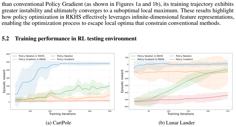
- [Section 5, Figures 1 and 2] The experimental section does not report the number of random seeds, error bars, or hyperparameter values (β, temperature T, kernel bandwidth, learning rate), so the claims of 'clear quadratic convergence' and 'superior performance' cannot be assessed from the figures alone.
- [Section 2.1, Eq. (1)] The definition of Ψ_t(τ) in the text uses γ^{i-1}, while Eq. (1) and the surrounding discussion use γ^{t-1}; the indexing should be made consistent.
Circularity Check
Theorem 3.3's equivalence is asserted by replacing the RKHS norm in Eq. (5) with the Euclidean norm in Eq. (7), so the analyzed finite-dimensional subproblem is not derived from the Representer Theorem.
-
self definitional
[Appendix B, derivation of Theorem 3.3 around Eq. (7)]
"The objective function in Equation (5) is: L(¯α) = ⟨∇h ˆJ (hk) , ¯hα⟩ + 1/2 ⟨∇²h ˆJ (hk) ◦ ¯hα, ¯hα⟩ + β/6 ∥¯α∥3 2. We derive the forms for the first two terms. The third term, β/6 ∥¯α∥3 2, directly uses the Euclidean norm of ¯α as stated in Equation (7)."
Equation (5) minimizes over h̄∈H_K with cubic term β/6∥h̄∥_H^3. Under the representer form h̄=Σ_i α_i K(x_i,·), the RKHS norm is ∥h̄∥_H=(α^T G α)^{1/2} with G_ij=K(x_i,x_j), not ∥α∥_2. Appendix B simply sets the third term to β/6∥α∥_2^3 'as stated in Equation (7)', so the claimed equality between (5) and (7) is imposed by definition, not obtained from the Representer Theorem; it holds only when G=I. Since Algorithm 1 solves the Euclidean-norm problem (7) via Newton-CG while Lemma C.1 and the Section 4 convergence/quadratic-rate proofs use the RKHS stationarity condition ∇hĴ+∇²Ĵ∘Δh+(β/2)∥Δh∥Δh=0, the entire theory-algorithm link rests on this unproved norm identification.
full rationale
The paper does not fit a parameter and then relabel it as a prediction, and its convergence lemmas are standard cubic-regularization arguments rather than self-citations. The one load-bearing circular move is in the reduction of Eq. (5) to Eq. (7): the cubic term in (5) is β/6∥h̄∥_H^3, and under the representer form h̄=Σα_i K(x_i,·) the RKHS norm is (α^T G α)^{1/2}; Appendix B simply writes β/6∥α∥_2^3 'as stated in Equation (7)'. Thus the advertised equivalence — the step that makes the method finite-dimensional and links Algorithm 1 to the Section 4 convergence proofs — is not a consequence of the Representer Theorem but an imposed norm identity that holds only for G=I. Because Lemma C.1 and the quadratic-rate proof are written for the RKHS stationarity condition while Algorithm 1 (Newton-CG in Appendix F) solves v+Hα+(β/2)∥α∥_2 α=0, the theorem's claimed equality is the construction that carries the entire paper. The empirical benchmarks are external and non-circular, but they do not repair the theory-algorithm gap. Score 6.
Assumptions & free parameters
free parameters (5)
- cubic regularization coefficient β =
not reported
- learning rate η =
not reported
- policy temperature T =
not reported
- kernel hyperparameters (e.g., RBF bandwidth) =
not reported
- conjugate gradient tolerance and max iterations =
tol=1e-3, maxiter=500
assumptions (5)
- domain assumption Lipschitz continuity of the RKHS Hessian with L ≤ β (Assumption 4.1)
- domain assumption Bounded variance of Monte Carlo gradient and Hessian estimates (Lemma 4.1)
- domain assumption Bounded inverse operator and small update step in Theorem 4.6
- standard math Representer Theorem applies to the cubic-regularized subproblem
- ad hoc to paper Euclidean norm of coefficients replaces the RKHS norm of the update in the cubic term
Cite this review
Pith. "Pith review of Policy Newton Algorithm in Reproducing Kernel Hilbert Space." pith.science (2026). https://pith.science/paper/IPWRSR7L
@misc{pith2026250601597,
  author       = {Pith},
  title        = {Pith review of: Policy Newton Algorithm in Reproducing Kernel Hilbert Space},
  year         = {2026},
  howpublished = {\url{https://pith.science/paper/IPWRSR7L}},
  note         = {Machine review of arXiv:2506.01597}
}
read the original abstract
Reinforcement learning (RL) policies represented in Reproducing Kernel Hilbert Spaces (RKHS) offer powerful representational capabilities. While second-order optimization methods like Newton's method demonstrate faster convergence than first-order approaches, current RKHS-based policy optimization remains constrained to first-order techniques. This limitation stems primarily from the intractability of explicitly computing and inverting the infinite-dimensional Hessian operator in RKHS. We introduce Policy Newton in RKHS, the first second-order optimization framework specifically designed for RL policies represented in RKHS. Our approach circumvents direct computation of the inverse Hessian operator by optimizing a cubic regularized auxiliary objective function. Crucially, we leverage the Representer Theorem to transform this infinite-dimensional optimization into an equivalent, computationally tractable finite-dimensional problem whose dimensionality scales with the trajectory data volume. We establish theoretical guarantees proving convergence to a local optimum with a local quadratic convergence rate. Empirical evaluations on a toy financial asset allocation problem validate these theoretical properties, while experiments on standard RL benchmarks demonstrate that Policy Newton in RKHS achieves superior convergence speed and higher episodic rewards compared to established first-order RKHS approaches and parametric second-order methods. Our work bridges a critical gap between non-parametric policy representations and second-order optimization methods in reinforcement learning.
Figures

Reference graph
Works this paper leans on
-
[1]
Practical kernel-based reinforcement learning
André MS Barreto, Doina Precup, and Joelle Pineau. Practical kernel-based reinforcement learning. Journal of Machine Learning Research, 17(67):1–70, 2016
work page 2016
-
[2]
Optimization methods for large-scale machine learning
Léon Bottou, Frank E Curtis, and Jorge Nocedal. Optimization methods for large-scale machine learning. SIAM Review, 60(2):223–311, 2018
2018
-
[3]
A tutorial on support vector machines for pattern recognition
Christopher JC Burges. A tutorial on support vector machines for pattern recognition. Data Mining and Knowledge Discovery, 2(2):121–167, 1998
work page 1998
-
[4]
Second-order kernel online convex optimization with adaptive sketching
Daniele Calandriello, Alessandro Lazaric, and Michal Valko. Second-order kernel online convex optimization with adaptive sketching. In International Conference on Machine Learning, pages 645–653, 2017
work page 2017
-
[5]
Efficient second-order online kernel learning with adaptive embedding
Daniele Calandriello, Alessandro Lazaric, and Michal Valko. Efficient second-order online kernel learning with adaptive embedding. Advances in Neural Information Processing Systems, 30, 2017
work page 2017
-
[6]
Super-universal regularized newton method
Nikita Doikov, Konstantin Mishchenko, and Yurii Nesterov. Super-universal regularized newton method. SIAM Journal on Optimization, 34(1):27–56, 2024
work page 2024
-
[7]
Approximate newton methods for policy search in markov decision processes
Thomas Furmston, Guy Lever, and David Barber. Approximate newton methods for policy search in markov decision processes. Journal of Machine Learning Research, 17(226):1–51, 2016
work page 2016
-
[8]
Stochastic first-and zeroth-order methods for nonconvex stochastic programming
Saeed Ghadimi and Guanghui Lan. Stochastic first-and zeroth-order methods for nonconvex stochastic programming. SIAM Journal on Optimization, 23(4):2341–2368, 2013
2013
Show all 41 references
-
[9]
Quasi-newton trust region policy optimization
Devesh K Jha, Arvind U Raghunathan, and Diego Romeres. Quasi-newton trust region policy optimization. In Conference on Robot Learning, pages 945–954, 2020
2020
-
[10]
Convergence and decomposition for tensor products of hilbert space operators
Carlos S Kubrusly and Paulo CM Vieira. Convergence and decomposition for tensor products of hilbert space operators. Operators and Matrices, 2(3):407–416, 2008
2008
-
[11]
The conjugate gradient method for optimal control problems
L Lasdon, S Mitter, and A Waren. The conjugate gradient method for optimal control problems. IEEE Transactions on Automatic Control, 12(2):132–138, 2003
2003
-
[12]
Fastfood-approximating kernel expansions in loglinear time
Quoc Le, Tamás Sarlós, Alex Smola, et al. Fastfood-approximating kernel expansions in loglinear time. In International Conference on Machine Learning, pages 244–252, 2013
2013
-
[13]
Dynamic asset allocation exploiting predictors in reinforcement learning framework
Jae Won Lee, Jongwoo Lee, Byoung-Tak Zhang, et al. Dynamic asset allocation exploiting predictors in reinforcement learning framework. In European Conference on Machine Learning, pages 298–309, 2004
2004
-
[14]
Parameterizing non-parametric meta- reinforcement learning tasks via subtask decomposition
Suyoung Lee, Myungsik Cho, and Youngchul Sung. Parameterizing non-parametric meta- reinforcement learning tasks via subtask decomposition. In Advances in Neural Information Processing Systems, volume 36, 2023
2023
-
[15]
Modelling policies in mdps in reproducing kernel hilbert space
Guy Lever and Ronnie Stafford. Modelling policies in mdps in reproducing kernel hilbert space. In Artificial intelligence and statistics, pages 590–598, 2015
2015
-
[16]
Approximate newton policy gradient algorithms
Haoya Li, Samarth Gupta, Hsiangfu Yu, Lexing Ying, and Inderjit Dhillon. Approximate newton policy gradient algorithms. SIAM Journal on Scientific Computing, 45(5):A2585–A2609, 2023
2023
-
[17]
Large scale online kernel learning
Jing Lu, Steven CH Hoi, Jialei Wang, Peilin Zhao, and Zhi-Yong Liu. Large scale online kernel learning. Journal of Machine Learning Research, 17(47):1–43, 2016
2016
-
[18]
A cubic-regularized policy newton algorithm for reinforcement learning
Mizhaan P Maniyar, LA Prashanth, Akash Mondal, and Shalabh Bhatnagar. A cubic-regularized policy newton algorithm for reinforcement learning. In International Conference on Artificial Intelligence and Statistics, pages 4708–4716. PMLR, 2024
2024
-
[19]
Methods for calculating fréchet derivatives and sensi- tivities for the non-linear inverse problem: A comparative study 1
Peter R Mcgillivray and DW Oldenburg. Methods for calculating fréchet derivatives and sensi- tivities for the non-linear inverse problem: A comparative study 1. Geophysical Prospecting, 38 (5):499–524, 1990. 10
1990
-
[20]
A scalable kernel approach to reinforcement learning
Jean-Marc Mercier, Aguirre Max, et al. A scalable kernel approach to reinforcement learning. SSRN, 2025
2025
-
[21]
Nonparametric return distribution approximation for reinforcement learning
Tetsuro Morimura, Masashi Sugiyama, Hisashi Kashima, Hirotaka Hachiya, and Toshiyuki Tanaka. Nonparametric return distribution approximation for reinforcement learning. In International Conference on Machine Learning, pages 799–806, 2010
2010
-
[22]
Universal approximation using radial-basis-function networks
Jooyoung Park and Irwin W Sandberg. Universal approximation using radial-basis-function networks. Neural Computation, 3(2):246–257, 1991
1991
-
[23]
Stochastic policy gradient ascent in Reproducing Kernel Hilbert Spaces
Santiago Paternain, Juan Andrés Bazerque, Austin Small, and Alejandro Ribeiro. Stochastic policy gradient ascent in Reproducing Kernel Hilbert Spaces. IEEE Transactions on Automatic Control, 66(8):3429–3444, 2020
2020
-
[24]
Policy gradient for continu- ing tasks in discounted markov decision processes
Santiago Paternain, Juan Andrés Bazerque, and Alejandro Ribeiro. Policy gradient for continu- ing tasks in discounted markov decision processes. IEEE Transactions on Automatic Control, 67(9):4467–4482, 2022
2022
-
[25]
A generalized representer theorem
Bernhard Schölkopf, Ralf Herbrich, and Alex J Smola. A generalized representer theorem. In International Conference on Computational Learning Theory, pages 416–426, 2001
2001
-
[26]
Hessian aided policy gradient
Zebang Shen, Alejandro Ribeiro, Hamed Hassani, Hui Qian, and Chao Mi. Hessian aided policy gradient. In International conference on machine learning, pages 5729–5738. PMLR, 2019
2019
-
[27]
Sutton and Andrew G
Richard S. Sutton and Andrew G. Barto. Reinforcement learning: an introduction. 2018
2018
-
[28]
Policy gradient meth- ods for reinforcement learning with function approximation
Richard S Sutton, David McAllester, Satinder Singh, and Yishay Mansour. Policy gradient meth- ods for reinforcement learning with function approximation. Advances in Neural Information Processing Systems, 12, 1999
1999
-
[29]
Mujoco: A physics engine for model-based control
Emanuel Todorov, Tom Erez, and Yuval Tassa. Mujoco: A physics engine for model-based control. In 2012 IEEE/RSJ International Conference on Intelligent Robots and Systems, pages 5026–5033, 2012
2012
-
[30]
Gymnasium: A standard interface for reinforcement learning environments
Mark Towers, Ariel Kwiatkowski, Jordan Terry, John U Balis, Gianluca De Cola, Tristan Deleu, Manuel Goulao, Andreas Kallinteris, Markus Krimmel, Arjun KG, et al. Gymnasium: A standard interface for reinforcement learning environments. arXiv preprint arXiv:2407.17032, 2024
2024 arXiv
-
[31]
On the convergence rates of policy gradient methods
Lin Xiao. On the convergence rates of policy gradient methods. Journal of Machine Learning Research, 23(282):1–36, 2022
2022
-
[32]
Safety aarl: Weight adjustment for reinforcement- learning-based safety dynamic asset allocation strategies
Seong Joon Yoo, Yeong Hyeon Gu, et al. Safety aarl: Weight adjustment for reinforcement- learning-based safety dynamic asset allocation strategies. Expert Systems with Applications, 227:120297, 2023
2023
-
[33]
Global convergence of policy gradient methods to (almost) locally optimal policies
Kaiqing Zhang, Alec Koppel, Hao Zhu, and Tamer Basar. Global convergence of policy gradient methods to (almost) locally optimal policies. SIAM Journal on Control and Optimization, 58 (6):3586–3612, 2020
2020
-
[34]
Residual kernel policy network: Enhancing stability and robustness in rkhs-based reinforcement learning
Yixian Zhang, Huaze Tang, Huijing Lin, and Wenbo Ding. Residual kernel policy network: Enhancing stability and robustness in rkhs-based reinforcement learning. In International Conference on Learning Representations, 2025. A The derivation of the second-order Fréchet derivativ...
2025
-
[35]
Let Xl(¯hα) = ⟨∇h log πh(xl), ¯hα⟩
Contribution from H (1) op : Let ∇h log πh(xl)(·) = T K(xl, ·) − Ea′∼π(·|sl) [K((sl, a′), ·)] . Let Xl(¯hα) = ⟨∇h log πh(xl), ¯hα⟩. Xl(¯hα) = T MX i=1 αi K(xl, xi) − Ea′∼π(·|sl) [K((sl, a′), xi)] The quadratic form from H (1) op is ⟨H (1) op ◦ ¯hα, ¯hα⟩ = PM l=1 Ψl(τ )Xl(¯hα) ...
-
[36]
The quadratic form is ⟨H (2) op ◦ ¯hα, ¯hα⟩ = PM l=1 Ψl(τ )T Cova′∼π(·|sl)[K((sl, a′), ·)] ◦ ¯hα, ¯hα
Contribution from H (2) op : H (2) op ◦ u = PM l=1 Ψl(τ )T Cova′∼π(·|sl)[K((sl, a′), ·)] ◦ u. The quadratic form is ⟨H (2) op ◦ ¯hα, ¯hα⟩ = PM l=1 Ψl(τ )T Cova′∼π(·|sl)[K((sl, a′), ·)] ◦ ¯hα, ¯hα . The inner term is Vara′∼π(·|sl)[⟨K((sl, a′), ·), ¯hα⟩] = ¯α⊤Σ(l) ¯α, where Σ(l)...
-
[37]
Resource Dynamics: The probability of resource level transitions depends on the chosen action: • Conservative strategy: P (rt+1|rt, at = 0) = [0 .1, 0.8, 0.1, 0.0, 0.0] for ∆r ∈ {−1, 0, +1, +2, +3} 24 • Balanced strategy: P (rt+1|rt, at = 1) = [0 .2, 0.2, 0.4, 0.2, 0.0] for ∆r...
-
[38]
Market Dynamics: Market state transitions follow a Markov chain with the following probabilities: • Recession: P (mt+1|mt = 0) = [0.6, 0.3, 0.1] for mt+1 ∈ {0, 1, 2} • Stability: P (mt+1|mt = 1) = [0.3, 0.4, 0.3] for mt+1 ∈ {0, 1, 2} • Prosperity: P (mt+1|mt = 2) = [0.1, 0.3, ...
-
[39]
The conjugate gradient method is employed to efficiently solve this linear system, avoiding the high computational cost of directly computing (H + β 2 ∥ ¯α∥I)−1
The objective function and its gradient are computed as: f ( ¯α) = ⟨v, ¯α⟩ + 1 2 ⟨H ¯α, ¯α⟩ + β 6 ∥ ¯α∥3 2 ∇f ( ¯α) = v + H ¯α + β 2 ∥ ¯α∥ ¯α In each Newton iteration, we determine the search direction by solving the linear system (H + β 2 ∥ ¯α∥I)∆ ¯α = −∇f ( ¯α). The conjugat...
-
[40]
Initialize residual r0 = −∇f ( ¯α0) = −(v + H ¯α0 + β 2 ∥ ¯α0∥ ¯α0) and initial search direction p0 = r0
-
[41]
To balance optimization accuracy and computational efficiency, we set the convergence tolerance to10−3 and the maximum number of iterations to 500
For each iteration k: • Compute optimal step size αk = rT k rk pT k (H+ β 2 ∥ ¯αk∥I)pk • Update solution ∆ ¯αk+1 = ∆ ¯αk + αkpk • Update residual rk+1 = rk − αk(H + β 2 ∥ ¯αk∥I)pk • Calculate conjugate direction update coefficient βk = rT k+1rk+1 rT k rk • Update search direct...
Reviewed August 7, 2026 · model on record in the stance chip above.
Discussion (0). Continue with ORCID to comment.