REVIEW 4 major objections 8 minor 92 references
Multimodal Spatiotemporal Atmospheric Data Assimilation with Latent Flow-matching
T0 review · 4 major / 8 minor · reviewed 2026-08-06 · deepseek-v4-flash
Pith's one-line read A single frozen weather-video prior performs filtering, smoothing, and forecasting by changing only which frames are observed.
desk verdict A serious, well-ablated empirical study of latent video flow-matching for atmospheric DA; the unified-prior claim mostly holds, but the posterior approximation is never checked against a reference and the GraphDOP comparison is curve-extracted. read the letter →
The pith
A machine-rendered reading of the paper's core claim, the machinery that carries it, and where it could break.
The reading
What carries the argument
The central object is the latent video flow-matching prior: a TrigFlow model (spherical interpolation between latent and Gaussian noise, $z_t = \cos(t) z_0 + \sin(t) \varepsilon$) trained on 128-channel autoencoder latents of 32-frame, 8-day ERA5 windows. At sampling time, a guided TrigFlow sampler combines the learned velocity with a DPS-style likelihood gradient evaluated at the Tweedie estimate of the clean latent, annealed by an SDA coefficient, plus a low-noise Langevin corrector, to draw posterior samples. The measurement operator $A$ (grid subsampling, bilinear interpolation at stations, or super-obbing) is the only thing that changes across tasks.
What would settle it
Run a classical ensemble or variational assimilation system (e.g., an ensemble Kalman filter or 4D-Var) on the same ERA5 truth and the same sparse IGRA/ISD observations, and compare RMSE and ensemble calibration on the withheld-station test; if the classical system beats the posterior at comparable or lower compute, the DPS-style likelihood approximation would be in doubt.
Extended reading notes
Core claim
The paper's central claim is that temporal consistency is internal to the prior: a latent video flow-matching model trained unconditionally on ERA5 windows propagates information from observed frames to unobserved frames, so the classical data-assimilation regimes (filtering, smoothing, fixed-interval reconstruction) reduce to choosing which temporal frames are observed. With real radiosonde (IGRA), surface station (ISD), and ship/buoy (ICOADS) observations, the same frozen prior reconstructs the full 69-variable atmospheric state and produces ensemble forecasts directly from observations, competitive at longer leads with GraphDOP, an observation-to-forecast system trained on a broader observing network. The authors also report that posterior samples remain geostrophically and hypsometrically consistent, and that ensemble spread is reasonably calibrated when the corrector noise is retained.
Load-bearing premise
The posterior sampler approximates the observation likelihood score using the gradient at the denoised (Tweedie) estimate with a hand-tuned annealing strength, and the paper never checks this approximation against a classical data-assimilation baseline.
Editorial extensions
If this is right
- The same frozen prior can realize the classical DA regimes—filter (leading frames observed), smoother (middle frames observed), and fixed-interval reconstruction—with no retraining, simply by changing the observed-frame mask.
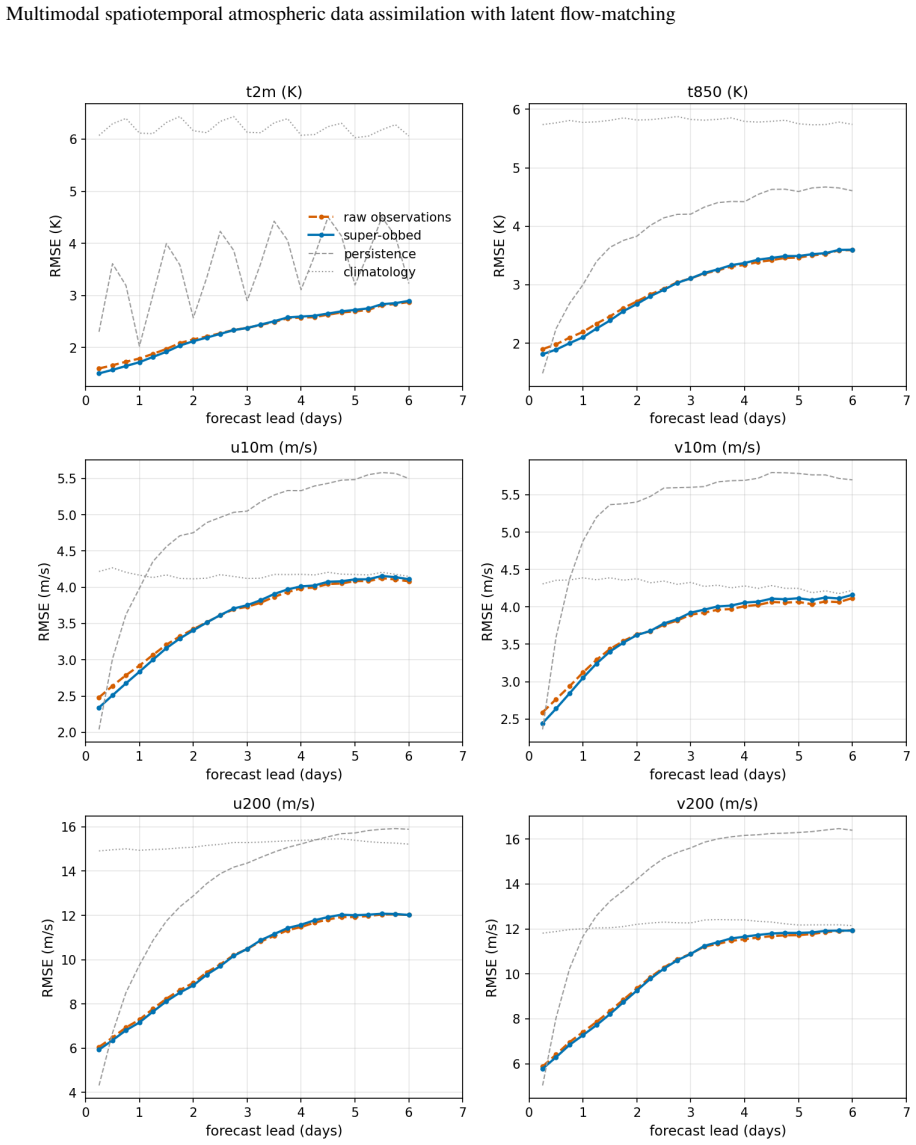
- Full-state ensemble forecasts can be generated directly from sparse real observations, with six-day forecast skill comparable to GraphDOP at long leads and better for 2 m temperature.
- The prior's internal temporal propagation replaces the separate emulator or numerical forecast model used in earlier snapshot-based generative DA.
- Ensemble spread from posterior draws provides uncertainty quantification, with SSR values 0.72–0.85 across tasks, underdispersed but in the right direction for operational inflation.
Reading between the lines
- A natural extension is to treat the observation mask as a user input, turning the same prior into an interactive tool for observing-system design: one could ask which frames or stations most reduce posterior spread. The paper does not test this.
- Because the likelihood operator is differentiable and the prior is video-based, the framework could in principle ingest future satellite radiances through a differentiable radiative-transfer operator, which the authors note is left to future work.
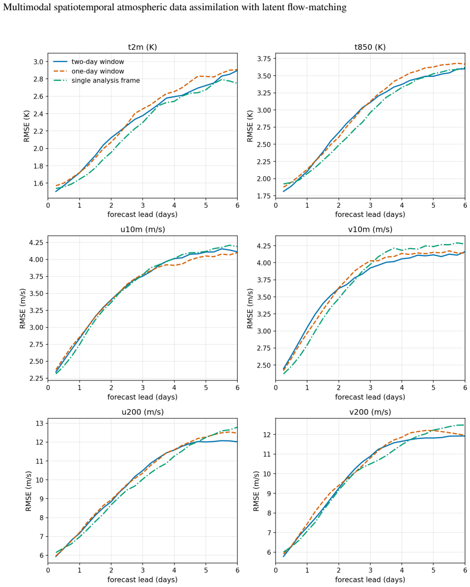
- The fact that observed-window length barely changed forecast skill (Appendix C) suggests the prior's internal dynamics, not the conditioning window, dominate the forecast; a testable implication is that even shorter windows than one frame may suffice for some applications.
Editorial analysis
A structured set of objections, weighed in public.
Referee Report
Summary. This paper trains a 3D autoencoder and a latent video flow-matching prior (TrigFlow with a DiT3D backbone) on 69-variable ERA5 windows of 32 six-hourly frames, then uses a guided sampler with a DPS-style likelihood and SDA annealing to condition this frozen prior on observations. The authors demonstrate super-resolution from coarse grids, data fusion from real IGRA and ISD station data, filtering/smoothing/fixed-interval regimes obtained by changing only which frames are observed, and direct observation-to-forecast for 2020, including a Hurricane Laura case study. The central claim is that one frozen generative video prior can act as the forecast model and likelihood in several classical DA configurations, with uncertainty quantified by the spread of posterior draws.
Significance. If the posterior samples are faithful, this is a substantial empirical contribution: a single generative prior supports multiple DA geometries and produces physically consistent states, with extensive ablations, held-out station verification, and released code. The authors are unusually transparent about limitations, including the absence of an end-to-end operational comparison and the explicitly illustrative Aardvark experiment (Appendix D). The main caveats are that the likelihood approximation is not validated against a reference posterior and that the GraphDOP comparison is not a same-protocol rerun; these issues are fixable and do not erase the value of the empirical study.
major comments (4)
- [Sec. 2.2-2.3, Eq. (6)-(7), Algorithm 1] The likelihood is not fully specified as a Bayesian posterior. The observation noise scale σ_y is introduced but never assigned a value; the guidance scale is task-dependent (e.g., scale 4.0 for SR vs 0.5 for station tasks in Table 13) and γ is tuned. In Algorithm 1 the gradient is multiplied by this hand-set scale, effectively tempering the likelihood. Because the abstract's core claim is that this is 'Bayesian inference' and 'posterior sampling', the paper should either report σ_y and a sensitivity analysis for the tuned constants, or validate the approximation against a reference posterior/classical DA scheme (e.g., an ensemble Kalman filter, a particle filter on a reduced problem, or a variational method). The comparisons in App. A.5 are against other approximate samplers (DAPS, DiffPIR, PnP-DM, STeP-HMC), none of which is a reference posterior. This is load-bearing for the headline claim of a unified DA approach.
- [Table 3] The calibration results show SSR 0.72-0.85 and empirical coverage around 0.77 versus the Gaussian target of 0.954 for 8-member ensembles. This is direct evidence that the posterior spread is overconfident, which weakens the claim that the method provides calibrated uncertainty quantification through ensemble spread. The authors note that an inflation-style correction would be needed, but the main text should either include such a correction and report the resulting SSR/coverage, or substantially qualify the UQ claims. As written, the uncertainty quantification contribution is only partially supported.
- [Sec. 4.4, Fig. 16] The GraphDOP and IFS skill curves are extracted from a published figure rather than obtained by running those models under the same protocol. The text states this, but the quantitative claims of being 'competitive with state-of-the-art observation-to-forecast models' and having 'clear advantages over GraphDOP at longer leads' rest on that extraction. There are no error bars or uncertainty estimates for the extracted curves, and GraphDOP uses a broader observing system. A same-protocol rerun (at least for GraphDOP) or a clearly labelled qualitative comparison with softened claims is needed.
- [Table 6] In the held-out station verification for IGRA, the reconstruction RMSE is consistently higher than ERA5 at the same withheld stations (e.g., t2m 3.16 vs 2.91 K, z500 165 vs 155 m2/s2, t300 1.42 vs 1.19 K, u200 3.77 vs 2.95 m/s). The sentence that the reconstruction 'closely tracks that of ERA5' understates this gap. The claim that the reconstruction is competitive with ERA5 in observation space should be revised or quantified, for example with ratios or confidence intervals.
minor comments (8)
- [Eq. (7)] Please state the value of σ_y used in each experiment; it is introduced as the observation noise standard deviation but no value is reported anywhere in the paper.
- [Fig. 16] Add a caption note stating that the GraphDOP and IFS curves are digitized from Ref. [28] and describe the extraction procedure so readers can assess the accuracy of the comparison.
- [Table 13] Report the guidance scale and γ values used for the station and observation-to-forecast tasks, not only for the SR sweep.
- [Introduction] The statement in Sec. 5 that 'an end-to-end comparison with operational assimilation is beyond our scope' is a useful caveat; consider moving it to the introduction so readers do not over-interpret the DA claims.
- [Appendix D] The Aardvark experiment is already flagged as illustrative, but the figure caption should also clearly say it uses a training-period observation and is not a held-out test.
- [App. A.5] The sentence that baseline performance 'reflects our implementations rather than the methods in general' is honest; please release the exact configurations for these baselines in the code repository to support reproducibility.
- [Fig. 1 caption] The phrase 'The latent video looks like Gaussian noise visually; however, it has some small structures' is informal; rephrase it in a more precise way.
- [Keywords] There is a missing space in 'KeywordsGenerative' at the start of the keyword line.
Circularity Check
The main DA chain is self-contained and non-circular; the only reduction found is a disclosed in-sample Aardvark illustration, which is minor and not load-bearing.
-
other
[Appendix D (Forecasting from the Aardvark latent observations), Fig. 27]
"The public Aardvark release contains only one observation data point, on 2018-08-18, (which falls within our training period). A held-out, multiple initial conditions test would require an extended observation-assembly pipeline, which we leave for future work. In this simplified experiment, we observe that the Aardvark latent lowers the forecast errors, with some variables performing better than GraphDOP."
This experiment feeds a latent observation from 2018-08-18, a date inside the 1979-2018 ERA5 training window, into the frozen prior and then verifies the resulting forecast against ERA5 for the same date. Because the prior was trained on ERA5 windows that include that date, the 'forecast' is not a strictly out-of-sample prediction; it could be produced by recall of seen states rather than by the claimed generalization of the latent video prior. The paper itself labels it 'just an illustration, not a rigorous test case benchmark' and does not use it to support the central observation-to-forecast comparisons, which are based on thirty-two disjoint 2020 initial conditions. The step is therefore a disclosed in-sample illustration rather than a load-bearing circular result.
full rationale
The paper's central derivation is not circular by construction. A frozen latent video prior is trained on ERA5 windows from 1979-2018, and all headline DA experiments condition on external observations via the likelihood of Eq. (6) and the annealed variance of Eq. (7); the observations enter through the measurement operator A, and the scoring is against held-out ERA5 frames or withheld station observations. The DPS-style likelihood at the Tweedie estimate is an approximation, and the paper does not validate it against a reference posterior, but that is a correctness and calibration concern, not a circular reduction. No fitted parameter is renamed as a prediction: the sampler hyperparameters are tuned on validation windows and applied to disjoint test initial conditions, and the GraphDOP comparison uses an external published benchmark. The only genuine reduction to training inputs is the Appendix D Aardvark forecast, which uses a training-period observation date and is explicitly described by the authors as an illustration, not a rigorous test; the main observation-to-forecast results in Sec. 4.4 are independent of it. Self-citations are present but not load-bearing: the cited prior work [22] is used only to contrast the snapshot approach with the present video prior. Overall, the derivation chain stands on its own, with one minor disclosed in-sample experiment preventing a zero score.
Assumptions & free parameters
free parameters (6)
- guidance scale (SR) =
4.0
- guidance scale (station tasks) =
0.5 with DSG
- SDA annealing coefficient gamma =
0.1
- corrector activation threshold sigma_c_max =
3 or 5
- corrector noise scale lambda =
0 or 1
- log-noise training distribution =
ln sigma ~ N(0,1.5^2), sigma in [0.002,80]
assumptions (6)
- standard math TrigFlow spherical interpolation, Tweedie estimate, and DPM-Solver++ rotation update are valid.
- ad hoc to paper The DPS likelihood gradient evaluated at the Tweedie estimate is a faithful approximation to the true posterior score for the measurement operators used.
- domain assumption Observation errors are Gaussian, independent, with known sigma_y, and the measurement operator A is differentiable.
- domain assumption ERA5 reanalysis is an acceptable ground truth for evaluation.
- domain assumption The frozen autoencoder decoder faithfully reconstructs all 69 physical variables from latents.
- domain assumption The learned 32-frame video distribution generalizes to the 2020 test period.
Cite this review
Pith. "Pith review of Multimodal Spatiotemporal Atmospheric Data Assimilation with Latent Flow-matching." pith.science (2026). https://pith.science/paper/IW2ZU27A
@misc{pith2026260805103,
  author       = {Pith},
  title        = {Pith review of: Multimodal Spatiotemporal Atmospheric Data Assimilation with Latent Flow-matching},
  year         = {2026},
  howpublished = {\url{https://pith.science/paper/IW2ZU27A}},
  note         = {Machine review of arXiv:2608.05103}
}
read the original abstract
Data assimilation (DA) uses Bayesian inference to update the state of a numerical forecast model with observed data. In this study, we propose a fundamentally different, unified approach to atmospheric data assimilation. We use latent video flow-matching to sample temporally consistent trajectories from a prior trained using ERA5 reanalysis (69 variables over an 8-day window). We also use posterior sampling to assimilate real observation sources, such as those from the NOAA Integrated Global Radiosonde Archive and the Integrated Surface Database. Because the prior generates a continuous trajectory, it naturally propagates information between observed and unobserved frames. Therefore, we can perform various DA tasks, such as filtering and smoothing, simply by changing the observed frames. Moreover, we generate full-state ensemble forecasts directly from sparse observations, achieving performance competitive with state-of-the-art observation-to-forecast models.
Figures


Figures from the paper (39 more)




Reference graph
Works this paper leans on
-
[1]
Toward unification of the multiscale modeling of the atmosphere.Atmospheric Chemistry and Physics, 11(8):3731–3742, 2011
A Arakawa, J-H Jung, and C-M Wu. Toward unification of the multiscale modeling of the atmosphere.Atmospheric Chemistry and Physics, 11(8):3731–3742, 2011
2011
-
[2]
Springer Science & Business Media, 2003
Horst J Neugebauer.Dynamics of multiscale earth systems, volume 97. Springer Science & Business Media, 2003
2003
-
[3]
Multiscale cloud system modeling.Reviews of Geophysics, 47(4), 2009
Wei-Kuo Tao and Mitchell W Moncrieff. Multiscale cloud system modeling.Reviews of Geophysics, 47(4), 2009
2009
-
[4]
Satellite data assimilation in numerical weather prediction: An overview
Jean-Noël Thépaut. Satellite data assimilation in numerical weather prediction: An overview. InProceedings of ECMWF Seminar on Recent Developments in Data Assimilation for Atmosphere and Ocean, ECMWF , Reading, UK, pages 8–12, 2003
2003
-
[5]
Observing-system experiments in the ecmwf 4d-var data assimilation system
François Bouttier and Graeme Kelly. Observing-system experiments in the ecmwf 4d-var data assimilation system. Quarterly Journal of the Royal Meteorological Society, 127(574):1469–1488, 2001
2001
-
[6]
A bayesian tutorial for data assimilation.Physica D: Nonlinear Phenomena, 230(1-2):1–16, 2007
Christopher K Wikle and L Mark Berliner. A bayesian tutorial for data assimilation.Physica D: Nonlinear Phenomena, 230(1-2):1–16, 2007
2007
-
[7]
Evaluating data assimilation algorithms.Monthly weather review, 140(11):3757–3782, 2012
Kody JH Law and Andrew M Stuart. Evaluating data assimilation algorithms.Monthly weather review, 140(11):3757–3782, 2012
2012
-
[8]
The era5 global reanalysis.Quarterly journal of the royal meteorological society, 146(730):1999–2049, 2020
Hans Hersbach, Bill Bell, Paul Berrisford, Shoji Hirahara, András Horányi, Joaquín Muñoz-Sabater, Julien Nicolas, Carole Peubey, Raluca Radu, Dinand Schepers, et al. The era5 global reanalysis.Quarterly journal of the royal meteorological society, 146(730):1999–2049, 2020
1999
Show all 92 references
-
[9]
World Scientific, 2014
Istvan Szunyogh.Applicable atmospheric dynamics: Techniques for the exploration of atmospheric dynamics. World Scientific, 2014
2014
-
[10]
Data assimilation and its applications.Proceedings of the National Academy of Sciences, 97(21):11143–11144, 2000
Bin Wang, Xiaolei Zou, and Jiang Zhu. Data assimilation and its applications.Proceedings of the National Academy of Sciences, 97(21):11143–11144, 2000
2000
-
[11]
Data assimilation methods in the earth sciences.Advances in water resources, 31(11):1411–1418, 2008
Rolf H Reichle. Data assimilation methods in the earth sciences.Advances in water resources, 31(11):1411–1418, 2008
2008
-
[12]
Learning deep generative models.Annual Review of Statistics and Its Application, 2(1):361–385, 2015
Ruslan Salakhutdinov. Learning deep generative models.Annual Review of Statistics and Its Application, 2(1):361–385, 2015
2015
-
[13]
Generative learning for forecasting the dynamics of high-dimensional complex systems.Nature Communications, 15(1):8904, 2024
Han Gao, Sebastian Kaltenbach, and Petros Koumoutsakos. Generative learning for forecasting the dynamics of high-dimensional complex systems.Nature Communications, 15(1):8904, 2024
2024
-
[14]
Probabilistic weather forecasting with machine learning.Nature, 637(8044):84–90, 2025
Ilan Price, Alvaro Sanchez-Gonzalez, Ferran Alet, Tom R Andersson, Andrew El-Kadi, Dominic Masters, Timo Ewalds, Jacklynn Stott, Shakir Mohamed, Peter Battaglia, et al. Probabilistic weather forecasting with machine learning.Nature, 637(8044):84–90, 2025
2025
-
[15]
Maximum likelihood training of score-based diffusion models.Advances in neural information processing systems, 34:1415–1428, 2021
Yang Song, Conor Durkan, Iain Murray, and Stefano Ermon. Maximum likelihood training of score-based diffusion models.Advances in neural information processing systems, 34:1415–1428, 2021
2021
-
[16]
Score-based generative modeling through stochastic differential equations.arXiv preprint arXiv:2011.13456, 2020
Yang Song, Jascha Sohl-Dickstein, Diederik P Kingma, Abhishek Kumar, Stefano Ermon, and Ben Poole. Score-based generative modeling through stochastic differential equations.arXiv preprint arXiv:2011.13456, 2020
2011 arXiv
-
[17]
Elucidating the design space of diffusion-based generative models.Advances in neural information processing systems, 35:26565–26577, 2022
Tero Karras, Miika Aittala, Timo Aila, and Samuli Laine. Elucidating the design space of diffusion-based generative models.Advances in neural information processing systems, 35:26565–26577, 2022
2022
-
[18]
Flow matching for generative modeling.arXiv preprint arXiv:2210.02747, 2022
Yaron Lipman, Ricky TQ Chen, Heli Ben-Hamu, Maximilian Nickel, and Matt Le. Flow matching for generative modeling.arXiv preprint arXiv:2210.02747, 2022
2022 arXiv
-
[19]
Scaling rectified flow transformers for high-resolution image synthesis
Patrick Esser, Sumith Kulal, Andreas Blattmann, Rahim Entezari, Jonas Müller, Harry Saini, Yam Levi, Dominik Lorenz, Axel Sauer, Frederic Boesel, et al. Scaling rectified flow transformers for high-resolution image synthesis. InForty-first international conference on machine l...
2024
-
[20]
Diffusion models as plug-and-play priors.Advances in Neural Information Processing Systems, 35:14715–14728, 2022
Alexandros Graikos, Nikolay Malkin, Nebojsa Jojic, and Dimitris Samaras. Diffusion models as plug-and-play priors.Advances in Neural Information Processing Systems, 35:14715–14728, 2022
2022
-
[21]
Diffusion posterior sampling for general noisy inverse problems.arXiv preprint arXiv:2209.14687, 2022
Hyungjin Chung, Jeongsol Kim, Michael T Mccann, Marc L Klasky, and Jong Chul Ye. Diffusion posterior sampling for general noisy inverse problems.arXiv preprint arXiv:2209.14687, 2022
2022 arXiv
-
[22]
Multimodal atmospheric super-resolution with deep generative models.Machine Learning: Earth, 2(1):015001, 2026
Dibyajyoti Chakraborty, Haiwen Guan, Jason Stock, Troy Arcomano, Guido Cervone, and Romit Maulik. Multimodal atmospheric super-resolution with deep generative models.Machine Learning: Earth, 2(1):015001, 2026. 25 Multimodal spatiotemporal atmospheric data assimilation with lat...
2026
-
[23]
Simplifying, stabilizing and scaling continuous-time consistency models
Cheng Lu and Yang Song. Simplifying, stabilizing and scaling continuous-time consistency models. InInterna- tional Conference on Learning Representations, volume 2025, pages 50611–50649, 2025
2025
-
[24]
Scalable diffusion models with transformers
William Peebles and Saining Xie. Scalable diffusion models with transformers. InProceedings of the IEEE/CVF international conference on computer vision, pages 4195–4205, 2023
2023
-
[25]
Overview of the integrated global radiosonde archive.Journal of Climate, 19(1):53–68, 2006
Imke Durre, Russell S V ose, and David B Wuertz. Overview of the integrated global radiosonde archive.Journal of Climate, 19(1):53–68, 2006
2006
-
[26]
The integrated surface database: Recent developments and partnerships
Adam Smith, Neal Lott, and Russ V ose. The integrated surface database: Recent developments and partnerships. Bulletin of the American Meteorological Society, 92(6):704–708, 2011
2011
-
[27]
Icoads release 3.0: a major update to the historical marine climate record.International Journal of Climatology, 37(5):2211–2232, 2017
Eric Freeman, Scott D Woodruff, Steven J Worley, Sandra J Lubker, Elizabeth C Kent, William E Angel, David I Berry, Philip Brohan, Ryan Eastman, Lydia Gates, et al. Icoads release 3.0: a major update to the historical marine climate record.International Journal of Climatology,...
2017
-
[28]
Graphdop: Towards skilful data-driven medium-range weather forecasts learnt and initialised directly from observations.arXiv preprint arXiv:2412.15687, 2024
Mihai Alexe, Eulalie Boucher, Peter Lean, Ewan Pinnington, Patrick Laloyaux, Anthony McNally, Simon Lang, Matthew Chantry, Chris Burrows, Marcin Chrust, et al. Graphdop: Towards skilful data-driven medium-range weather forecasts learnt and initialised directly from observation...
2024 arXiv
-
[29]
Super-resolution reconstruction of turbulent flows with machine learning.Journal of Fluid Mechanics, 870:106–120, 2019
Kai Fukami, Koji Fukagata, and Kunihiko Taira. Super-resolution reconstruction of turbulent flows with machine learning.Journal of Fluid Mechanics, 870:106–120, 2019
2019
-
[30]
Super-resolution and denoising of 4d-flow mri using physics-informed deep neural nets
Mojtaba F Fathi, Isaac Perez-Raya, Ahmadreza Baghaie, Philipp Berg, Gabor Janiga, Amirhossein Arzani, and Roshan M D’Souza. Super-resolution and denoising of 4d-flow mri using physics-informed deep neural nets. Computer Methods and Programs in Biomedicine, 197:105729, 2020
2020
-
[31]
Physics-informed cnns for super-resolution of sparse observa- tions on dynamical systems.arXiv preprint arXiv:2210.17319, 2022
Daniel Kelshaw, Georgios Rigas, and Luca Magri. Physics-informed cnns for super-resolution of sparse observa- tions on dynamical systems.arXiv preprint arXiv:2210.17319, 2022
2022 arXiv
-
[32]
Super-resolution analysis via machine learning: a survey for fluid flows.Theoretical and Computational Fluid Dynamics, 37(4):421–444, 2023
Kai Fukami, Koji Fukagata, and Kunihiko Taira. Super-resolution analysis via machine learning: a survey for fluid flows.Theoretical and Computational Fluid Dynamics, 37(4):421–444, 2023
2023
-
[33]
Super-resolution and denoising of fluid flow using physics-informed convolutional neural networks without high-resolution labels.Physics of Fluids, 33(7), 2021
Han Gao, Luning Sun, and Jian-Xun Wang. Super-resolution and denoising of fluid flow using physics-informed convolutional neural networks without high-resolution labels.Physics of Fluids, 33(7), 2021
2021
-
[34]
Physr: Physics-informed deep super-resolution for spatiotemporal data.Journal of Computational Physics, 492:112438, 2023
Pu Ren, Chengping Rao, Yang Liu, Zihan Ma, Qi Wang, Jian-Xun Wang, and Hao Sun. Physr: Physics-informed deep super-resolution for spatiotemporal data.Journal of Computational Physics, 492:112438, 2023
2023
-
[35]
Single-snapshot machine learning for super-resolution of turbulence.Journal of Fluid Mechanics, 1001:A32, 2024
Kai Fukami and Kunihiko Taira. Single-snapshot machine learning for super-resolution of turbulence.Journal of Fluid Mechanics, 1001:A32, 2024
2024
-
[36]
Mesh-based super-resolution of fluid flows with multiscale graph neural networks
Shivam Barwey, Pinaki Pal, Saumil Patel, Riccardo Balin, Bethany Lusch, Venkatram Vishwanath, Romit Maulik, and Ramesh Balakrishnan. Mesh-based super-resolution of fluid flows with multiscale graph neural networks. Computer Methods in Applied Mechanics and Engineering, 443:118...
2025
-
[37]
Global field reconstruction from sparse sensors with voronoi tessellation-assisted deep learning.Nature Machine Intelligence, 3(11):945–951, 2021
Kai Fukami, Romit Maulik, Nesar Ramachandra, Koji Fukagata, and Kunihiko Taira. Global field reconstruction from sparse sensors with voronoi tessellation-assisted deep learning.Nature Machine Intelligence, 3(11):945–951, 2021
2021
-
[38]
Probabilistic neural networks for fluid flow surrogate modeling and data recovery.Physical Review Fluids, 5(10):104401, 2020
Romit Maulik, Kai Fukami, Nesar Ramachandra, Koji Fukagata, and Kunihiko Taira. Probabilistic neural networks for fluid flow surrogate modeling and data recovery.Physical Review Fluids, 5(10):104401, 2020
2020
-
[39]
Quantifying uncertainty for deep learning based forecasting and flow-reconstruction using neural architecture search ensembles.Physica D: Nonlinear Phenomena, 454:133852, 2023
Romit Maulik, Romain Egele, Krishnan Raghavan, and Prasanna Balaprakash. Quantifying uncertainty for deep learning based forecasting and flow-reconstruction using neural architecture search ensembles.Physica D: Nonlinear Phenomena, 454:133852, 2023
2023
-
[40]
Averaging weights leads to wider optima and better generalization.arXiv preprint arXiv:1803.05407, 2018
Pavel Izmailov, Dmitrii Podoprikhin, Timur Garipov, Dmitry Vetrov, and Andrew Gordon Wilson. Averaging weights leads to wider optima and better generalization.arXiv preprint arXiv:1803.05407, 2018
2018 arXiv
-
[41]
Assessments of epistemic uncertainty using gaussian stochastic weight averaging for fluid-flow regression.Physica D: Nonlinear Phenomena, 440:133454, 2022
Masaki Morimoto, Kai Fukami, Romit Maulik, Ricardo Vinuesa, and Koji Fukagata. Assessments of epistemic uncertainty using gaussian stochastic weight averaging for fluid-flow regression.Physica D: Nonlinear Phenomena, 440:133454, 2022
2022
-
[42]
Deep unsupervised learning using nonequilibrium thermodynamics
Jascha Sohl-Dickstein, Eric Weiss, Niru Maheswaranathan, and Surya Ganguli. Deep unsupervised learning using nonequilibrium thermodynamics. InInternational conference on machine learning, pages 2256–2265. pmlr, 2015
2015
-
[43]
Denoising diffusion probabilistic models.Advances in neural information processing systems, 33:6840–6851, 2020
Jonathan Ho, Ajay Jain, and Pieter Abbeel. Denoising diffusion probabilistic models.Advances in neural information processing systems, 33:6840–6851, 2020
2020
-
[44]
Generative modeling by estimating gradients of the data distribution.Advances in neural information processing systems, 32, 2019
Yang Song and Stefano Ermon. Generative modeling by estimating gradients of the data distribution.Advances in neural information processing systems, 32, 2019. 26 Multimodal spatiotemporal atmospheric data assimilation with latent flow-matching
2019
-
[45]
Estimation of non-normalized statistical models by score matching.Journal of Machine Learning Research, 6(4), 2005
Aapo Hyvärinen. Estimation of non-normalized statistical models by score matching.Journal of Machine Learning Research, 6(4), 2005
2005
-
[46]
Flow straight and fast: Learning to generate and transfer data with rectified flow.arXiv preprint arXiv:2209.03003, 2022
Xingchao Liu, Chengyue Gong, and Qiang Liu. Flow straight and fast: Learning to generate and transfer data with rectified flow.arXiv preprint arXiv:2209.03003, 2022
2022 arXiv
-
[47]
Stochastic interpolants: A unifying framework for flows and diffusions.Journal of Machine Learning Research, 26(209):1–80, 2025
Michael Albergo, Nicholas M Boffi, and Eric Vanden-Eijnden. Stochastic interpolants: A unifying framework for flows and diffusions.Journal of Machine Learning Research, 26(209):1–80, 2025
2025
-
[48]
Pseudoinverse-guided diffusion models for inverse problems
Jiaming Song, Arash Vahdat, Morteza Mardani, and Jan Kautz. Pseudoinverse-guided diffusion models for inverse problems. InInternational conference on learning representations, 2023
2023
-
[49]
Denoising diffusion restoration models.Advances in neural information processing systems, 35:23593–23606, 2022
Bahjat Kawar, Michael Elad, Stefano Ermon, and Jiaming Song. Denoising diffusion restoration models.Advances in neural information processing systems, 35:23593–23606, 2022
2022
-
[50]
Zero-shot image restoration using denoising diffusion null-space model
Yinhuai Wang, Jiwen Yu, and Jian Zhang. Zero-shot image restoration using denoising diffusion null-space model. arXiv preprint arXiv:2212.00490, 2022
2022 arXiv
-
[51]
A variational perspective on solving inverse problems with diffusion models
Morteza Mardani, Jiaming Song, Jan Kautz, and Arash Vahdat. A variational perspective on solving inverse problems with diffusion models. InInternational Conference on Learning Representations, volume 2024, pages 28027–28053, 2024
2024
-
[52]
Denoising diffusion models for plug-and-play image restoration
Yuanzhi Zhu, Kai Zhang, Jingyun Liang, Jiezhang Cao, Bihan Wen, Radu Timofte, and Luc Van Gool. Denoising diffusion models for plug-and-play image restoration. InProceedings of the IEEE/CVF conference on computer vision and pattern recognition, pages 1219–1229, 2023
2023
-
[53]
Principled probabilistic imaging using diffusion models as plug-and-play priors.Advances in Neural Information Processing Systems, 37:118389–118427, 2024
Zihui Wu, Yu Sun, Yifan Chen, Bingliang Zhang, Yisong Yue, and Katherine L Bouman. Principled probabilistic imaging using diffusion models as plug-and-play priors.Advances in Neural Information Processing Systems, 37:118389–118427, 2024
2024
-
[54]
Improving diffusion inverse problem solving with decoupled noise annealing
Bingliang Zhang, Wenda Chu, Julius Berner, Chenlin Meng, Anima Anandkumar, and Yang Song. Improving diffusion inverse problem solving with decoupled noise annealing. InProceedings of the Computer Vision and Pattern Recognition Conference, pages 20895–20905, 2025
2025
-
[55]
Solving linear inverse problems provably via posterior sampling with latent diffusion models.Advances in Neural Information Processing Systems, 36:49960–49990, 2023
Litu Rout, Negin Raoof, Giannis Daras, Constantine Caramanis, Alex Dimakis, and Sanjay Shakkottai. Solving linear inverse problems provably via posterior sampling with latent diffusion models.Advances in Neural Information Processing Systems, 36:49960–49990, 2023
2023
-
[56]
Solving inverse problems with latent diffusion models via hard data consistency
Bowen Song, Soo Min Kwon, Zecheng Zhang, Xinyu Hu, Qing Qu, and Liyue Shen. Solving inverse problems with latent diffusion models via hard data consistency. InInternational Conference on Learning Representations, volume 2024, pages 7624–7654, 2024
2024
-
[57]
Inversebench: Benchmarking plug-and-play diffusion priors for inverse problems in physical sciences
Hongkai Zheng, Wenda Chu, Bingliang Zhang, Zihui Wu, Austin Wang, Berthy Feng, Caifeng Zou, Yu Sun, Nikola Kovachki, Zachary Ross, et al. Inversebench: Benchmarking plug-and-play diffusion priors for inverse problems in physical sciences. InInternational Conference on Learning...
2025
-
[58]
Residual corrective diffusion modeling for km-scale atmospheric downscaling.Communications Earth & Environment, 6(1):124, 2025
Morteza Mardani, Noah Brenowitz, Yair Cohen, Jaideep Pathak, Chieh-Yu Chen, Cheng-Chin Liu, Arash Vahdat, Mohammad Amin Nabian, Tao Ge, Akshay Subramaniam, et al. Residual corrective diffusion modeling for km-scale atmospheric downscaling.Communications Earth & Environment, 6(...
2025
-
[59]
Precipitation downscaling with spatiotemporal video diffusion.Advances in Neural Information Processing Systems, 37:56374–56400, 2024
Prakhar Srivastava, Ruihan Yang, Gavin Kerrigan, Gideon Dresdner, Jeremy McGibbon, Christopher Bretherton, and Stephan Mandt. Precipitation downscaling with spatiotemporal video diffusion.Advances in Neural Information Processing Systems, 37:56374–56400, 2024
2024
-
[60]
Generative diffusion-based downscaling for climate.arXiv preprint arXiv:2404.17752, 2024
Robbie A Watt and Laura A Mansfield. Generative diffusion-based downscaling for climate.arXiv preprint arXiv:2404.17752, 2024
2024 arXiv
-
[61]
Generative emulation of weather forecast ensembles with diffusion models.Science Advances, 10(13):eadk4489, 2024
Lizao Li, Robert Carver, Ignacio Lopez-Gomez, Fei Sha, and John Anderson. Generative emulation of weather forecast ensembles with diffusion models.Science Advances, 10(13):eadk4489, 2024
2024
-
[62]
Continuous ensemble weather forecasting with diffusion models
Martin Andrae, Tomas Landelius, Joel Oskarsson, and Fredrik Lindsten. Continuous ensemble weather forecasting with diffusion models. InInternational Conference on Learning Representations, volume 2025, pages 26392– 26416, 2025
2025
-
[63]
Diffda: a diffusion model for weather-scale data assimilation.arXiv preprint arXiv:2401.05932, 2024
Langwen Huang, Lukas Gianinazzi, Yuejiang Yu, Peter D Dueben, and Torsten Hoefler. Diffda: a diffusion model for weather-scale data assimilation.arXiv preprint arXiv:2401.05932, 2024
2024 arXiv
-
[64]
Generative data assimilation of sparse weather station observations at kilometer scales.Journal of Advances in Modeling Earth Systems, 17(10):e2024MS004505, 2025
Peter Manshausen, Yair Cohen, Peter Harrington, Jaideep Pathak, Mike Pritchard, Piyush Garg, Morteza Mardani, Karthik Kashinath, Simon Byrne, and Noah Brenowitz. Generative data assimilation of sparse weather station observations at kilometer scales.Journal of Advances in Mode...
2025
-
[65]
Generative assimilation and prediction for weather and climate.arXiv preprint arXiv:2503.03038, 2025
Shangshang Yang, Congyi Nai, Xinyan Liu, Weidong Li, Jie Chao, Jingnan Wang, Leyi Wang, Xichen Li, Xi Chen, Bo Lu, et al. Generative assimilation and prediction for weather and climate.arXiv preprint arXiv:2503.03038, 2025
2025 arXiv
-
[66]
Deep generative data assimilation in multimodal setting
Yongquan Qu, Juan Nathaniel, Shuolin Li, and Pierre Gentine. Deep generative data assimilation in multimodal setting. InProceedings of the IEEE/CVF conference on computer vision and pattern recognition, pages 449–459, 2024
2024
-
[67]
Phyda: Physics-guided diffusion models for data assimilation in atmospheric systems.arXiv preprint arXiv:2505.12882, 2025
Hao Wang, Jindong Han, Wei Fan, Weijia Zhang, and Hao Liu. Phyda: Physics-guided diffusion models for data assimilation in atmospheric systems.arXiv preprint arXiv:2505.12882, 2025
2025 arXiv
-
[68]
A score-based filter for nonlinear data assimilation.Journal of Computational Physics, 514:113207, 2024
Feng Bao, Zezhong Zhang, and Guannan Zhang. A score-based filter for nonlinear data assimilation.Journal of Computational Physics, 514:113207, 2024
2024
-
[69]
Ensemble score filter with image inpainting for data assimilation in tracking surface quasi-geostrophic dynamics with partial observations.arXiv preprint arXiv:2501.12419, 2025
Siming Liang, Hoang Tran, Feng Bao, Hristo G Chipilski, Peter Jan van Leeuwen, and Guannan Zhang. Ensemble score filter with image inpainting for data assimilation in tracking surface quasi-geostrophic dynamics with partial observations.arXiv preprint arXiv:2501.12419, 2025
2025 arXiv
-
[70]
Step: A framework for solving scientific video inverse problems with spatiotemporal diffusion priors.arXiv preprint arXiv:2504.07549, 2025
Bingliang Zhang, Zihui Wu, Berthy T Feng, Yang Song, Yisong Yue, and Katherine L Bouman. Step: A framework for solving scientific video inverse problems with spatiotemporal diffusion priors.arXiv preprint arXiv:2504.07549, 2025
2025 arXiv
-
[71]
Appa: Bending weather dynamics with latent diffusion models for global data assimilation.arXiv preprint arXiv:2504.18720, 2025
Gérôme Andry, Sacha Lewin, François Rozet, Omer Rochman, Victor Mangeleer, Matthias Pirlet, Elise Faulx, Marilaure Grégoire, and Gilles Louppe. Appa: Bending weather dynamics with latent diffusion models for global data assimilation.arXiv preprint arXiv:2504.18720, 2025
2025
-
[72]
Tweedie’s formula and selection bias.Journal of the American Statistical Association, 106(496):1602–1614, 2011
Bradley Efron. Tweedie’s formula and selection bias.Journal of the American Statistical Association, 106(496):1602–1614, 2011
2011
-
[73]
Analyzing and improving the training dynamics of diffusion models
Tero Karras, Miika Aittala, Jaakko Lehtinen, Janne Hellsten, Timo Aila, and Samuli Laine. Analyzing and improving the training dynamics of diffusion models. InProceedings of the IEEE/CVF conference on computer vision and pattern recognition, pages 24174–24184, 2024
2024
-
[74]
Classifier-free diffusion guidance.arXiv preprint arXiv:2207.12598, 2022
Jonathan Ho and Tim Salimans. Classifier-free diffusion guidance.arXiv preprint arXiv:2207.12598, 2022
2022 arXiv
-
[75]
Score-based data assimilation.Advances in Neural Information Processing Systems, 36:40521–40541, 2023
François Rozet and Gilles Louppe. Score-based data assimilation.Advances in Neural Information Processing Systems, 36:40521–40541, 2023
2023
-
[76]
Dpm-solver++: Fast solver for guided sampling of diffusion probabilistic models.Machine Intelligence Research, 22(4):730–751, 2025
Cheng Lu, Yuhao Zhou, Fan Bao, Jianfei Chen, Chongxuan Li, and Jun Zhu. Dpm-solver++: Fast solver for guided sampling of diffusion probabilistic models.Machine Intelligence Research, 22(4):730–751, 2025
2025
-
[77]
Traversing distortion-perception tradeoff using a single score-based generative model
Yuhan Wang, Suzhi Bi, Ying-Jun Angela Zhang, and Xiaojun Yuan. Traversing distortion-perception tradeoff using a single score-based generative model. InProceedings of the Computer Vision and Pattern Recognition Conference, pages 2377–2386, 2025
2025
-
[78]
Adaptive guidance: Training-free acceleration of conditional diffusion models
Angela Castillo, Jonas Kohler, Juan C Pérez, Juan Pablo Pérez, Albert Pumarola, Bernard Ghanem, Pablo Arbeláez, and Ali Thabet. Adaptive guidance: Training-free acceleration of conditional diffusion models. InProceedings of the AAAI Conference on Artificial Intelligence, volum...
1962
-
[79]
Guidance with spherical gaussian constraint for conditional diffusion.arXiv preprint arXiv:2402.03201, 2024
Lingxiao Yang, Shutong Ding, Yifan Cai, Jingyi Yu, Jingya Wang, and Ye Shi. Guidance with spherical gaussian constraint for conditional diffusion.arXiv preprint arXiv:2402.03201, 2024
2024 arXiv
-
[80]
A global three-dimensional multivariate statistical interpolation scheme.Monthly Weather Review, 109(4):701–721, 1981
AC Lorenc. A global three-dimensional multivariate statistical interpolation scheme.Monthly Weather Review, 109(4):701–721, 1981
1981
-
[81]
Tilo Ochotta, Christoph Gebhardt, Dietmar Saupe, and Werner Wergen. Adaptive thinning of atmospheric observations in data assimilation with vector quantization and filtering methods.Quarterly Journal of the Royal Meteorological Society: A journal of the atmospheric sciences, a...
2005
-
[82]
Weatherbench: a benchmark data set for data-driven weather forecasting.Journal of Advances in Modeling Earth Systems, 12(11):e2020MS002203, 2020
Stephan Rasp, Peter D Dueben, Sebastian Scher, Jonathan A Weyn, Soukayna Mouatadid, and Nils Thuerey. Weatherbench: a benchmark data set for data-driven weather forecasting.Journal of Advances in Modeling Earth Systems, 12(11):e2020MS002203, 2020
2020
-
[83]
Adam: A method for stochastic optimization.arXiv preprint arXiv:1412.6980, 2014
Diederik P Kingma and Jimmy Ba. Adam: A method for stochastic optimization.arXiv preprint arXiv:1412.6980, 2014
2014 arXiv
-
[84]
Decoupled weight decay regularization.arXiv preprint arXiv:1711.05101, 2017
Ilya Loshchilov and Frank Hutter. Decoupled weight decay regularization.arXiv preprint arXiv:1711.05101, 2017
2017 arXiv
-
[85]
A fixed-lag kalman smoother for retrospective data assimilation.Monthly Weather Review, 122(12):2838–2867, 1994
Stephen E Cohn, NS Sivakumaran, and Ricardo Todling. A fixed-lag kalman smoother for retrospective data assimilation.Monthly Weather Review, 122(12):2838–2867, 1994. 28 Multimodal spatiotemporal atmospheric data assimilation with latent flow-matching
1994
-
[86]
End-to-end data-driven weather prediction
Anna Allen, Stratis Markou, Will Tebbutt, James Requeima, Wessel P Bruinsma, Tom R Andersson, Michael Herzog, Nicholas D Lane, Matthew Chantry, J Scott Hosking, et al. End-to-end data-driven weather prediction. Nature, 641(8065):1172–1179, 2025
2025
-
[87]
Healda: Highlighting the importance of initial errors in end-to-end ai weather forecasts.arXiv preprint arXiv:2601.17636, 2026
Aayush Gupta, Akshay Subramaniam, Michael S Pritchard, Karthik Kashinath, Sergey Frolov, Kelsey Lieberman, Christopher Miller, Nicholas Silverman, and Noah D Brenowitz. Healda: Highlighting the importance of initial errors in end-to-end ai weather forecasts.arXiv preprint arXi...
2026 arXiv
-
[88]
Applying guidance in a limited interval improves sample and distribution quality in diffusion models.Advances in Neural Information Processing Systems, 37:122458–122483, 2024
Tuomas Kynkäänniemi, Miika Aittala, Tero Karras, Samuli Laine, Timo Aila, and Jaakko Lehtinen. Applying guidance in a limited interval improves sample and distribution quality in diffusion models.Advances in Neural Information Processing Systems, 37:122458–122483, 2024
2024
-
[89]
Sdedit: Guided image synthesis and editing with stochastic differential equations.arXiv preprint arXiv:2108.01073, 2021
Chenlin Meng, Yutong He, Yang Song, Jiaming Song, Jiajun Wu, Jun-Yan Zhu, and Stefano Ermon. Sdedit: Guided image synthesis and editing with stochastic differential equations.arXiv preprint arXiv:2108.01073, 2021
2021 arXiv
-
[90]
Restart sampling for improving generative processes.Advances in Neural Information Processing Systems, 36:76806–76838, 2023
Yilun Xu, Mingyang Deng, Xiang Cheng, Yonglong Tian, Ziming Liu, and Tommi Jaakkola. Restart sampling for improving generative processes.Advances in Neural Information Processing Systems, 36:76806–76838, 2023
2023
-
[91]
The effect of thinning and superobservations in a simple one-dimensional data analysis with mischaracterized error.Monthly Weather Review, 146(4):1181–1195, 2018
Ross N Hoffman. The effect of thinning and superobservations in a simple one-dimensional data analysis with mischaracterized error.Monthly Weather Review, 146(4):1181–1195, 2018
2018
-
[92]
Learning skillful medium-range global weather forecasting.Science, 382(6677):1416–1421, 2023
Remi Lam, Alvaro Sanchez-Gonzalez, Matthew Willson, Peter Wirnsberger, Meire Fortunato, Ferran Alet, Suman Ravuri, Timo Ewalds, Zach Eaton-Rosen, Weihua Hu, et al. Learning skillful medium-range global weather forecasting.Science, 382(6677):1416–1421, 2023. 29 Multimodal spati...
2023
Reviewed August 6, 2026 · model on record in the stance chip above.
Discussion (0). Sign in to comment.