Double Quantum Magnetometry at Large Static Magnetic Fields

C. Munuera-Javaloy; E. Solano; I. Arrazola; J. Casanova

REVIEW 2 major objections 4 minor 48 references

Double Quantum Magnetometry at Large Static Magnetic Fields

T0 review · 2 major / 4 minor · reviewed 2026-08-14 · deepseek-v4-flash

Challenge this review Re-run · record.json Download PDF Read on arXiv ↗ Review JSON

Pith's one-line read Tailored microwave envelopes restore full double-quantum magnetometry signal at large static fields.

desk verdict The idea is worth one serious look, but the key inversion equation in the Supplemental Material is wrong, so the central claim isn't established. read the letter →

arxiv 1908.06142 v3 pith:JKZK5IKW submitted 2019-08-16 quant-ph cond-mat.mes-hall

C. Munuera-Javaloy , I. Arrazola , E. Solano , J. Casanova This is my paper · ORCID

classification quant-phcond-mat.mes-hall

keywords doublequantummagnetometrynitrogen-vacancycentersnanoscaleNMRchemicalshiftmicrowavepulseshapingdynamicaldecouplinghigh-fieldsensingstroboscopiccontrol

verification ladder T0 review T1 audit T2 compute T3 formal

The pith

A machine-rendered reading of the paper's core claim, the machinery that carries it, and where it could break.

The reading

This paper presents a microwave-control protocol that makes double quantum magnetometry (DQM) practical at large static magnetic fields, the regime where chemical shifts in nuclear samples are largest and most useful. In DQM at high field, the usual three-pulse sequence flips the electron spin of a nitrogen-vacancy sensor, but finite-width $\pi$ pulses make the effective sensor-nucleus coupling coefficient $f_l$ drop sharply, so the signal nearly vanishes. The authors design a time-dependent Rabi frequency $\Omega(t)$ whose modulation cancels the unwanted integrals accumulated during each pulse, recovering the ideal value $f_l = (-1)^{(l-1)/2} 4/(\pi l)$ even though each pulse lasts several Larmor periods. The result is DQM at $B_z = 3$ T with a peak Rabi frequency of only about $(2\pi)\times 40$ MHz, larger signal contrast than single quantum magnetometry, and no inhomogeneous broadening that could be mistaken for a chemical shift.

What carries the argument

The load-bearing object is the modulation function $F(t)$ that the spin operator $S_z$ acquires under the three-pulse sequences, together with the envelope recovered from it as $\Omega(t) = d/dt\,\arccos[F(t)]$. For each finite-width $\pi$ pulse, $F(t)$ is written as the top-hat pulse contribution plus a Gaussian-windowed cosine, and the amplitude of that cosine is fixed so that $\int F(s)\cos(l\omega_D s)\,ds$ vanishes over the pulse interval; the free-evolution windows then combine to yield $|f_l| = 4/(\pi l)$ exactly when $t_\pi = nT/(3l)$. This cancellation is what converts realistic long pulses into effective instantaneous ones.

What would settle it

Drive a single-proton or few-proton sample at $B_z = 3$ T with the designed $\Omega(t)$, and tune the pulse duration $t_\pi$ around the predicted value $t_\pi = nT/(3l)$ while monitoring the DQM resonance peak; if the peak height follows $\cos((f_l/2)A_x t_f)$ with $f_l = 4/(\pi l)$ across that sweep and stays fixed when the envelope amplitude is scaled by a few percent, the central claim is supported, and if it drops or shifts, the cancellation is not hardware-tolerant.

Watch

Extended reading notes

Core claim

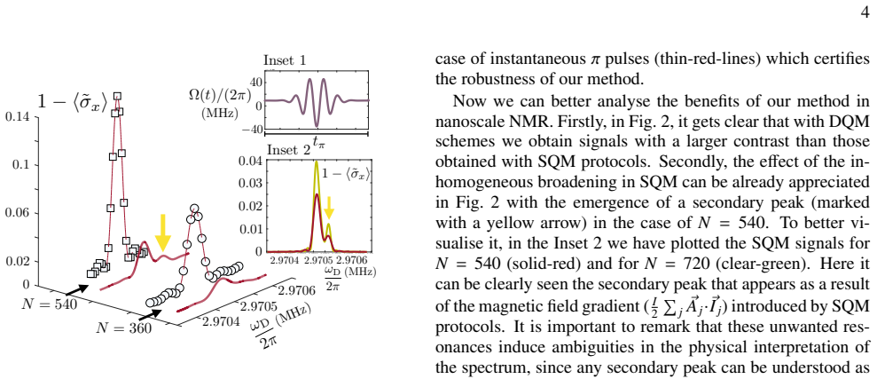
The central claim is that the DQM signal loss at large $B_z$ is not a fundamental limit but a pulse-shaping problem. Using a tailored envelope $\Omega(t)$ for the three-pulse sequences $\tilde{U}^{[+1,-1,+1]}_{[\pi,0]}$ and $\tilde{U}^{[-1,+1,-1]}_{[\pi,\pi/2]}$, the modulation function $F(t)$ of the $S_z$ operator is built so that the harmonic integrals over each finite-width pulse cancel; only the free-evolution intervals contribute, giving $f_l = 4/(\pi l)\,\cos(\pi\, 3t_\pi/(T/l))\,\sin(\pi l/2)$, which reaches the ideal magnitude $4/(\pi l)$ when the pulse duration obeys $t_\pi = nT/(3l)$. In numerical simulations with a five-proton cluster at 3 T, this recovers the ideal instantaneous-pulse signal, is stable against a 1% microwave amplitude error and a $(2\pi)\times 20$ kHz transition shift, and produces no secondary spectral peaks of the kind SQM generates through its field gradient.

Load-bearing premise

The protocol stands on the assumption that the microwave hardware can faithfully generate the designed envelope $\Omega(t)$ (equivalently $F(t)$) with the specified Gaussian width $\sigma_1$ and modulation index $k$; the paper does not state the exact parameter values used in its Fig. 2 simulation, so deviations such as finite rise times, phase transients, or amplitude calibration errors would degrade the cancellation and the recovered $f_l$ in a way the single simulated error scenario does not quantify.

Editorial extensions

If this is right

DQM can be run at 3 T with peak Rabi frequency about $(2\pi)\times 40$ MHz, instead of the very large microwave power that truly instantaneous pulses would require.
The ideal coupling coefficient $f_l = (-1)^{(l-1)/2}4/(\pi l)$ is restored, so the nanoscale NMR signal amplitude matches the instantaneous-pulse prediction rather than the much weaker finite-width value.
Because the method creates no magnetic-field gradient on the sample, the spectrum contains no secondary peaks that could be misread as chemical shifts.
The construction is not tied to the NV center's specific level structure, so it transfers to other quantum sensors and to other stroboscopic dynamical-decoupling sequences.

Reading between the lines

Editorial extensions of the paper, not claims the author makes directly.

The paper simulates a single 1% amplitude error and a fixed transition shift; a systematic sweep of envelope errors (rise time, phase transients, calibration of $\sigma_1$ and $k$) would tell how accurately the cancellation holds in hardware.
Because the same harmonic-cancellation idea applies to any sequence where finite pulse width attenuates a Fourier coefficient, it may transfer to XY-family or other DD sequences used in nanoscale NMR, a step the paper only hints at by saying the protocol is general.
Combining this high-field DQM with quantum-memory or clock-synchronized readout could push spectral resolution further, since the protocol already removes the gradient broadening that most limits interpretation.
An experiment that measures the DQM resonance peak height as $t_\pi$ is tuned across $t_\pi = nT/(3l)$ would directly test the predicted recovery curve $|f_l| = 4/(\pi l)$.

Share X Bluesky LinkedIn Reddit HN

Signed reviews

No signed human review yet.

Editorial analysis

A structured set of objections, weighed in public.

Desk editor's note, referee report, and a circularity audit.

Desk Editor's Note

read the letter

Interesting idea, but the central construction has a concrete mathematical error. The paper proposes tailoring the Rabi envelope Ω(t) to restore the ideal DQM Fourier coefficient f_l = 4/(πl) at large static fields, which is a practically relevant capability for NV-based nanoscale NMR. The three-pulse DQM building block is known, and the finite-pulse degradation of f_l was already noted for SQM, but the specific modulated Ω(t) that cancels the pulse-interval integrals is new. The paper also does a genuinely honest job simulating the full Hamiltonian (Eq. 6) rather than the effective model, and comparing to the analytic cos(f_43 A_x t/2) signal. The demonstration that SQM produces an inhomogeneous-broadening secondary peak while DQM does not is a clear and useful point.

The soft spot is not just missing parameters; it is a load-bearing error in the Supplemental Material. Eq. (S28) states Ω(t) = ∂_t arccos[F(t)], but their own Eq. (S30) defines F = 1/2(cos^2 φ + 1) with φ = ∫Ω/2 dt. Inverting that correctly gives Ω = 2 d/dt arccos(√(2F − 1)) (up to branch), not arccos(F). For a top-hat pulse the correct Ω is constant, while their formula gives zero at the edges and a nonconstant envelope. So the paper as written does not establish that the designed Ω(t) generates the required F(t), and the numerical validation cannot be trusted because no parameters (σ1, k, α1, n) or code are given. This is a considerable flaw because the entire protocol rests on that inversion.

The rest of the derivation—the three-pulse F(t) shapes, the Fourier-coefficient calculation, and the tπ condition—appears coherent, and the underlying idea may well be correct if the simulations used the proper inversion. But the manuscript as it stands fails to make the central claim reproducible.

This paper deserves a serious referee because the experimental target (DQM at 3 T for chemical-shift-enhanced nanoscale NMR) is important and the approach is not obviously wrong in spirit. It needs major revision: fix the inversion formula, report the actual simulation parameters, and ideally release the simulation code. I would not cite it in its current form.

Referee Report

2 major / 4 minor

Summary. The paper proposes a protocol for double quantum magnetometry (DQM) at large static magnetic fields, with nitrogen-vacancy centers as the primary example. The central idea is to use three-pulse sequences Ũ[+1,−1,+1] and Ũ[−1,+1,−1] to realize effective π rotations on the S_z operator, and then to tailor the microwave Rabi envelope Ω(t) so that the Fourier coefficient f_l of the resulting modulation function F(t) recovers the ideal instantaneous-pulse value f_l = (−1)^((l−1)/2) 4/(πl) even when the π pulses extend over several Larmor periods. The authors derive the modulation function F(t) for top-hat pulses, show that finite-width pulses reduce f_l, and then construct a modified F(t) with a Gaussian correction intended to cancel the pulse-interval integrals. Numerical simulations of the full Hamiltonian (6) are compared with the expected signal cos(f_43 A_x t/2), showing agreement for a 5-spin proton cluster at B_z = 3 T with moderate microwave power. The paper also emphasizes that DQM avoids the inhomogeneous broadening that appears in single quantum magnetometry.

Significance. If the central construction is correct, the protocol addresses a real and important limitation: DQM at large static fields currently requires either instantaneous pulses (and hence very high power) or suffers a severe reduction of the effective NV–nucleus coupling. Recovering the ideal f_l with finite-width pulses at moderate power, while avoiding inhomogeneous broadening, would make high-field nanoscale NMR with NV centers substantially more practical. The paper has clear strengths: the three-pulse-sequence derivation in the Supplemental Material is explicit and coherent; the numerical validation integrates the full Hamiltonian of Eq. (6), not merely the effective model, and compares against the independent expectation cos(f_l A_x t/2); and the claimed robustness to 1% amplitude errors and a 20 kHz energy shift is directly tested. However, the load-bearing step that converts the desired modulation function F(t) into a physical Rabi envelope Ω(t) is written incorrectly in Eq. (S28), and the simulation parameters for the tailored envelope are not reported. These issues prevent the central claim from being considered established as written, although they appear fixable.

major comments (2)

[Supplemental Material, Sec. IV, Eq. (S28)] The inversion from F(t) to Ω(t) is not correct as written. From Eq. (S30), F(t) = (1/2)(cos^2 φ(t) + 1) with φ(t) = ∫ Ω(s)/2 ds. Solving for φ gives φ = ± arccos(√(2F−1)), so Ω = 2 d/dt arccos(√(2F−1)) (with appropriate branch choices). Eq. (S28) instead states Ω(t) = ∂_t arccos[F(t)]. These differ: for the top-hat pulse shape F(t) = (1/2)[cos^2(π(t−t1)/tπ) + 1], the correct inversion yields the constant Ω = 2π/tπ, whereas Eq. (S28) gives a nonconstant envelope that vanishes at the pulse edges. Because the cancellation of the pulse integrals in Eq. (S22) relies on the F(t) actually generated by Ω(t), the derivation that one recovers f_l = (−1)^((l−1)/2) 4/(πl) is not mathematically supported. Please correct the inversion formula and show the resulting Ω(t) explicitly, or clarify if the symbol F(t) in Eq. (S28) means something different from the coefficient in Eq. (S30).
[Main text, Sec. III, Fig. 2; Supplemental Sec. IV] The numerical confirmation of the central claim is not reproducible from the information given. The tailored envelope in Fig. 2 is generated using the parameters k, σ1, α1, and the integer n in Eq. (S25), but none of these values is reported; the only stated quantities are tπ ≈ 0.16 μs and max Ω/(2π) ≈ 40 MHz. In particular, the amplitude α1 of the Gaussian correction is defined through Eq. (S27) and must be evaluated for each of the three pulse types in the sequences, yet no numerical values are provided. Without these parameters, or released simulation code, the reader cannot verify that the pulse-interval integrals in Eq. (S22) are actually cancelled, which is the key step in recovering the ideal f_l. Please provide the full set of parameters used in Fig. 2 (k, σ1, α1 for each pulse, n, and the timing offsets) or make the simulation code available.

minor comments (4)

[Main text, Sec. II, Fig. 1(d)] There is an apparent typo in the description of the finite-width top-hat simulation: the text states "The associated f31≈−0.0158 coefficient is marked in Fig. 1(c) with a yellow diamond", but the simulation is performed at the l = 43 resonance and the expected finite-width value quoted in the caption is f43 = −0.0118. The symbol "f31" should be "f43" and the numerical value should match the blue-diamond entry in the caption.
[Main text, around Eq. (12)] The sentence "for odd k, and top-hat π pulses" should presumably read "for odd l", since Eq. (12) defines f_l(r) and the subsequent discussion concerns l = 37 and l = 43.
[Main text, Fig. 1(c)] In Fig. 1(c), the labels f37 and f43 are placed near the curves, but it is hard to distinguish the two curves in the printed figure; adding a legend or an inset listing the exact values would improve clarity.
[Supplemental Material, Sec. II, Eqs. (S19)–(S20)] The formulas for f43 and the general f_l are stated with a particular sign convention; it would be clearer to present the general expression first and then specialize to l = 43, so that the sign of f43 in Eq. (S19) is immediately transparent.

Circularity Check

0 steps flagged · score 0.0 of 10

No significant circularity: the tailored-pulse construction is validated by full-Hamiltonian simulation against an independent analytic signal, not by restating its design inputs.

full rationale

The paper’s central construction is not circular. It first derives the modulation function F(t) from the toggling-frame evolution of S_z during each three-pulse sequence (Supplemental Eqs. S5–S17), then proposes an engineered F(t) whose Gaussian correction amplitude α1 is chosen to cancel the pulse-interval harmonic integrals in Eq. (S22). The target coefficient f_l = 4/(πl) is obtained from the remaining free-evolution integrals in Eq. (S23)–(S25); it is not taken as an input or fitted parameter. The designed Rabi envelope Ω(t) is then obtained by inverting the relation between F(t) and the pulse phase (Eqs. S29–S30). The numerical validation in Fig. 2 integrates the full spin Hamiltonian of Eq. (6), without assuming the effective model, and compares the resulting signal with the independent theoretical expectation cos(f_43 A_x t / 2) from Eq. (S21). That agreement is an external check on the construction, not a restatement of it. References to the authors’ earlier large-static-field work (Refs. 39–41) motivate the problem and are not used to justify the new protocol’s performance. No uniqueness theorem is imported, and no parameter is renamed as a prediction. The formula in Eq. (S28) may raise a correctness concern about the inversion, but that is not a circularity issue. Therefore the derivation is self-contained with respect to its claimed prediction.

Assumptions & free parameters 4 free parameters · 6 assumptions · 0 invented entities

No new physical entities are introduced. The central claim rests on the chosen pulse parameters, the standard NV spin-nucleus Hamiltonian, and the rotating-wave approximation. The most significant unstated inputs are the exact envelope parameters used in the numerical simulation.

free parameters (4)

Target harmonic l in simulations = 43
The demonstration is pinned to the 43rd harmonic of the pulse sequence, with 43 omega_D = omega_L at B_z = 3 T. The protocol is general, but the shown recovery depends on this choice.
Pulse duration t_pi = about 0.16 microsecond (about 20 Larmor periods)
Chosen to keep the maximum Rabi frequency near (2 pi) times 40 MHz, demonstrating moderate MW power. The cancellation construction requires a specific relation t_pi = n T / (3 l).
Gaussian width sigma1 in Eq. (S26) = not reported
The Supplemental Material says sigma1 can be freely adjusted, but the value used in the Fig. 2 simulation is not given, leaving the pulse envelope incompletely specified.
Modulation index k in Eq. (S26) = not reported
Sets the frequency of the oscillating Gaussian component used to cancel the pulse-interval harmonic integrals. The value used in the simulations is not stated, and Eq. (S27) requires a non-zero denominator.

assumptions (6)

domain assumption The NV center is described by the spin-1 Hamiltonian in Eq. (1) with zero-field splitting D, Zeeman term, and microwave driving coupled only to adjacent spin levels in the rotating frame.
The paper starts from this standard NV-center model without deriving it.
standard math The rotating-wave approximation is applied to the microwave driving in passing from Eq. (1) to Eq. (2).
Counter-rotating terms are dropped. This is standard and valid when the Rabi frequency is much smaller than the transition frequency, but it is not explicitly stated in the paper.
domain assumption The NV-nucleus interaction has the form S_z sum_j A_j dot I_j, with no nuclear-nuclear coupling and no electric quadrupole terms.
Used in Eq. (5) and in all simulations. It is adequate for the 13C/1H samples discussed but restricts generality.
domain assumption During the repeated sequence, the system is described by the toggling-frame Hamiltonian Eq. (9) with modulation function F(t) on S_z, expandable as a sum of even harmonics.
This is the basis for the resonance condition l omega_D = omega_L and for the f_l coefficients, so the entire pulse design rests on it.
domain assumption The initial nuclear state is approximated by the identity operator, i.e., the high-temperature limit.
Supplemental Eq. (S21) sets the nuclear initial state to 1/2 I, valid for room-temperature nuclear Zeeman energies but an approximation.
domain assumption The simulated target is a 5-spin hydrogen cluster with specified hyperfine vectors and no internuclear couplings.
Used for the numerical demonstrations in Sec. III; real samples may have different geometries, densities, and internuclear couplings.

how reviews work

0 comments

Cite this review

Pith. "Pith review of Double Quantum Magnetometry at Large Static Magnetic Fields." pith.science (2026). https://pith.science/paper/JKZK5IKW

@misc{pith2026190806142,
  author       = {Pith},
  title        = {Pith review of: Double Quantum Magnetometry at Large Static Magnetic Fields},
  year         = {2026},
  howpublished = {\url{https://pith.science/paper/JKZK5IKW}},
  note         = {Machine review of arXiv:1908.06142}
}

read the original abstract

We present a protocol to achieve double quantum magnetometry at large static magnetic fields. This is a regime where sensitive sample parameters, such as the chemical shift, get enhanced facilitating their characterization. In particular, our method delivers two-tone stroboscopic radiation patterns with modulated Rabi frequencies to achieve larger spectral signals. Furthermore, it does not introduce inhomogeneous broadening in the sample spectrum preventing signal misinterpretation. Moreover, our protocol is designed to work under realistic conditions such as the presence of moderate microwave power and errors on the radiation fields. Albeit we particularise to nitrogen vacancy centers, our protocol is general, thus applicable to distinct quantum sensors.

Figures

Figures reproduced from arXiv: 1908.06142 by the authors.

**Figure 2.** FIG. 2. Solid-red curves (wide curves) corresponds to ideal SQM [PITH_FULL_IMAGE:figures/full_fig_p004_2.png] view at source ↗

Discussion (0). Continue with ORCID to comment.

Reference graph

Works this paper leans on

48 extracted references · 46 canonical work pages

[1]

C. L. Degen, F. Reinhard, and P. Cappellaro, Rev. Mod. Phys. 89 , 035002 (2017)

2017
[2]

M. W. Doherty, N. B. Manson, P. Delaney, F. Jelezko, J. Wrachtrup, and L. C. L. Hollenberg, Phys. Rep. 528 , 1 (2013)

work page 2013
[3]

V. V. Dobrovitski, G. D. Fuchs, A. L. Falk, C. Santori, and D.D. Awschalom, Annu. Rev. Condens. Matter Phys. 4 , 23 (2013)

work page 2013
[4]

Rondin, J

L. Rondin, J. P. Tetienne, T. Hingant, J. F. Roch, P. Maletinsky, and V. Jacques, Rep. Prog. Phys. 77 , 056503 (2014)

work page 2014
[5]

Schirhagl, K

R. Schirhagl, K. Chang, M. Loretz, and C. L. Degen. Annu. Rev. Phys. Chem. 65 , 83 (2014)

work page 2014
[6]

Y. Wu, F. Jelezko, M. B. Plenio, and T. Weil, Angew. Chem. 55 , 6586 (2016)

work page 2016
[7]

A. M. Souza, G. A. \'Alvarez, and D. Suter, Phil. Trans. R. Soc. A 370 , 4748 (2012)

work page 2012
[8]

S. R. Hartmann and E. L. Hahn, Phys. Rev. 128 , 2042 (1962)

work page 1962

Show all 48 references

[9]

A. A. Maudsley, J. Magn. Reson. 69 , 488 (1986)

1986
[10]

Gullion, D

T. Gullion, D. B. Baker, and M. S. Conradi, J. Magn. Reson. 89 , 479 (1990)

1990
[11]

A. M. Souza, G. A. \'Alvarez, and D. Suter, Phys. Rev. Lett. 106 , 240501 (2011)

2011
[12]

Casanova, Z.-Y

J. Casanova, Z.-Y. Wang, J. F. Haase, and M. B. Plenio, Phys. Rev. A 92 , 042304 (2015)

2015
[13]

Z.-Y. Wang, J. Casanova, and M. B. Plenio, Nat. Commun. 8 , 14660 (2017)

2017
[14]

J. E. Lang, J. Casanova, Z.-Y. Wang, M. B. Plenio, and T. S. Monteiro, Phys. Rev. Applied 7 , 054009 (2017)

2017
[15]

Arrazola, J

I. Arrazola, J. Casanova, J. S. Pedernales, Z.-Y. Wang, E. Solano, and M. B. Plenio, Phys. Rev. A 97 , 052312 (2018)

2018
[16]

J. M. Taylor, P. Cappellaro, L. Childress, L. Jiang, D. Budker, P. R. Hemmer, A. Yacoby, R. Walsworth, and M. D. Lukin, Nat. Phys. 4 , 810 (2008)

2008
[17]

Kolkowitz, Q

S. Kolkowitz, Q. P. Unterreithmeier, S. D. Bennett, and M. D. Lukin, Phys. Rev. Lett. 109 , 137601 (2012)

2012
[18]

T. H. Taminiau, J. J. T. Wagenaar, T. van der Sar, F. Jelezko, V. V. Dobrovitski, and R. Hanson, Phys. Rev. Lett. 109 , 137602 (2012)

2012
[19]

N. Zhao, J. Honert, B. Schmid, M. Klas, J. Isoya, M. Markham, D. Twitchen, F. Jelezko, R.-B. Liu, H. Fedder, and J. Wrachtrup, Nat. Nanotech. 7 , 657 (2012)

2012
[20]

London, J

P. London, J. Scheuer, J.-M. Cai, I. Schwarz, A. Retzker, M. B. Plenio, M. Katagiri, T. Teraji, S. Koizumi, J. Isoya, R. Fischer, L. P. McGuinness, B. Naydenov, and F. Jelezko, Phys. Rev. Lett. 111 , 067601 (2013)

2013
[21]

Zopes, K

J. Zopes, K. Herb, K. S. Cujia, and C. L. Degen, Phys. Rev. Lett. 121 , 170801 (2018)

2018
[22]

Zopes, K

J. Zopes, K. S. Cujia, K. Sasaki, J. M. Boss, K. M. Itoh, and C. L. Degen, Nat. Commun. 9 , 4678 (2018)

2018
[23]

C. E. Bradley, J. Randall, M. H. Abobeih, R. C. Berrevoets, M. J. Degen, M. A. Bakker, M. Markham, D. J. Twitchen, and T. H. Taminiau, Phys. Rev. X 9 , 031045 (2019)

2019
[24]

M. H. Abobeih, J. Randall, C. E. Bradley, H. P. Bartling, M. A. Bakker, M. J. Degen, M. Markham, D. J. Twitchen, and T. H. Taminiau, Nature 576 , 411 (2019)

2019
[25]

H. J. Mamin, M. Kim, M. H. Sherwood, C. T. Rettner, K. Ohno, D. D. Awschalom, and D. Rugar, Science 339 , 557 (2013)

2013
[26]

Staudacher, F

T. Staudacher, F. Shi, S. Pezzagna, J. Meijer, J. Du, C. A. Meriles, F. Reinhard, and J. Wrachtrup, Science 339 , 561 (2013)

2013
[27]

M\" u ller, X

C. M\" u ller, X. Kong, J.-M. Cai, K. Melentijevi\'c, A. Stacey, M. Markham, D. Twitchen, J. Isoya, S. Pezzagna, J. Meijer, J. F. Du, M. B. Plenio, B. Naydenov, L. P. McGuinness, and F. Jelezko, Nat. Commun. 5 , 4703 (2014)

2014
[28]

F. Shi, Q. Zhang, P. Wang, H. Sun, J. Wang, X. Rong, M. Chen, C. Ju, F. Reinhard, H. Chen, J. Wrachtrup, J. Wang, and J. Du, Science 347 , 1135 (2015)

2015
[29]

Lovchinsky, A

I. Lovchinsky, A. O. Sushkov, E. Urbach, N. P. de Leon, S. Choi, K. De Greve, R. Evans, R. Gertner, E. Bersin, C. M\" u ller, L. McGuinness, F. Jelezko, R. L. Walsworth, H. Park, and M. D. Lukin, Science 351 , 836 (2016)

2016
[30]

Aslam, M

N. Aslam, M. Pfender, P. Neumann, R. Reuter, A. Zappe, F. F. de Oliveira, A. Denisenko, H. Sumiya, S. Onoda, J. Isoya, and J. Wrachtrup, Science 357 , 67 (2017)

2017
[31]

S. J. DeVience, L. M. Pham, I. Lovchinsky, A. O. Sushkov, N. Bar-Gill, C. Belthangady, F. Casola, M. Corbett, H. Zhang, M. Lukin, H. Park, A. Yacoby, and R. L. Walsworth, Nat. Nanotech. 10 , 129 (2015)

2015
[32]

D. R. Glenn, D. B. Bucher, J. Lee, M. D. Lukin, H. Park, and R. L. Walsworth, Nature 555 , 351 (2018)

2018
[33]

Rosskopf, J

T. Rosskopf, J. Zopes, J. M. Boss, and C. L. Degen, npj Quantum Information 3 , 33 (2017)

2017
[34]

u rner, T. Unden, G. Wolff, C. M\

S. Schmitt, T. Gefen, F. M. St\" u rner, T. Unden, G. Wolff, C. M\" u ller, J. Scheuer, B. Naydenov, M. Markham, S. Pezzagna, J. Meijer, I. Schwarz, M. Plenio, A. Retzker, L. P. McGuinness, and F. Jelezko, Science 356 , 832 (2017)

2017
[35]

J. M. Boss, K. S. Cujia, J. Zopes, C. L. Degen, Science 356 , 837 (2017)

2017
[36]

Reinhard, F

F. Reinhard, F. Shi, N. Zhao, F. Rempp, B. Naydenov, J. Meijer, L. T. Hall, L. Hollenberg, J. Du, R.-B. Liu, and J. Wrachtrup, Phys. Rev. Lett. 108 , 200402 (2012)

2012
[37]

K. Fang, V. M. Acosta, C. Santori, Z. Huang, K. M. Itoh, H. Watanabe, S. Shikata, and R. G. Beausoleil, Phys. Rev. Lett. 110 , 130802 (2013)

2013
[38]

H. J. Mamin, M. H. Sherwood, M. Kim, C. T. Rettner, K. Ohno, D. D. Awschalom, and D. Rugar, Phys. Rev. Lett. 113 , 030803 (2014)

2014
[39]

Casanova, Z.-Y

J. Casanova, Z.-Y. Wang, I. Schwartz, and M. B. Plenio, Phys. Rev. Applied 10 , 044072 (2018)

2018
[40]

Casanova, E

J. Casanova, E. Torrontegui, M. B. Plenio, J. J. Garc\' i a-Ripoll, and E. Solano, Phys. Rev. Lett. 122 , 010407 (2019)

2019
[41]

Arrazola, E

I. Arrazola, E. Solano, and J. Casanova, Phys. Rev. B 99 , 245405 (2019)

2019
[42]

M. H. Levitt, Spin Dynamics: Basics of Nuclear Magnetic Resonance (Wiley, West Sussex, 2008)

2008
[43]

E. C. Reynhardt and G. L. High, Prog. Nucl. Magn. Reson. Spectrosc. 38 , 37 (2001)

2001
[44]

See Supplemental Material for further details
[45]

Allard and T

P. Allard and T. H\" a rd, Journal of Magnetic Resonance 153 , 15 (2001)

2001
[46]

J. R. Maze, J. M. Taylor, and M. D. Lukin, Phys. Rev. B 78 , 094303 (2008)

2008
[47]

Casanova, Z.-Y

J. Casanova, Z.-Y. Wang, and M. B. Plenio, Phys. Rev. A 96 , 032314 (2017)

2017
[48]

Allard and T

P. Allard and T. H\" a rd Journal of Magnetic Resonance 153 , 15 (2001)

2001

Pith tools

Reviewed August 14, 2026 · model on record in the stance chip above.

[1] [1]

C. L. Degen, F. Reinhard, and P. Cappellaro, Rev. Mod. Phys. 89 , 035002 (2017)

2017

[2] [2]

M. W. Doherty, N. B. Manson, P. Delaney, F. Jelezko, J. Wrachtrup, and L. C. L. Hollenberg, Phys. Rep. 528 , 1 (2013)

work page 2013

[3] [3]

V. V. Dobrovitski, G. D. Fuchs, A. L. Falk, C. Santori, and D.D. Awschalom, Annu. Rev. Condens. Matter Phys. 4 , 23 (2013)

work page 2013

[4] [4]

Rondin, J

L. Rondin, J. P. Tetienne, T. Hingant, J. F. Roch, P. Maletinsky, and V. Jacques, Rep. Prog. Phys. 77 , 056503 (2014)

work page 2014

[5] [5]

Schirhagl, K

R. Schirhagl, K. Chang, M. Loretz, and C. L. Degen. Annu. Rev. Phys. Chem. 65 , 83 (2014)

work page 2014

[6] [6]

Y. Wu, F. Jelezko, M. B. Plenio, and T. Weil, Angew. Chem. 55 , 6586 (2016)

work page 2016

[7] [7]

A. M. Souza, G. A. \'Alvarez, and D. Suter, Phil. Trans. R. Soc. A 370 , 4748 (2012)

work page 2012

[8] [8]

S. R. Hartmann and E. L. Hahn, Phys. Rev. 128 , 2042 (1962)

work page 1962