REVIEW 3 major objections 5 minor 1 cited by
Bayesian Inference for Large Scale Image Classification
T0 review · 3 major / 5 minor · reviewed 2026-08-14 · deepseek-v4-flash
Pith's one-line read ATMC, an adaptive-noise MCMC sampler, is claimed to beat tuned SGD on ImageNet by sampling the posterior rather than optimizing the loss.
desk verdict First MCMC-on-ImageNet result with a genuinely new adaptive thermostat, but the printed integrator contradicts the paper's own SDE and the posterior-sampling claim collapses as written. read the letter →
The pith
A machine-rendered reading of the paper's core claim, the machinery that carries it, and where it could break.
The reading
What carries the argument
The load-bearing mechanism is the adaptive thermostat: a scalar control variate ξ per parameter, coupled to momentum through friction β(ξ)=α(ξ)+ξ with α(ξ)=max(D−ξ,0). The energy function H(θ,p,ξ)=L(θ)+K(p)+½(ξ−diag(B)/(2m))² and specially chosen dynamics D and Q make the mini-batch noise covariance B cancel out of the continuous-time equation, leaving a noise-robust Langevin dynamics. The momentum energy K(p) can be Gaussian or hyperbolic, and the hyperbolic form bounds the maximum parameter update per step. The numerical machinery is a two-way Strang-split integrator whose momentum substep solves the Ornstein–Uhlenbeck process exactly, so gradient and noise terms are damped by friction before being applied.
What would settle it
Run ATMC on a small Bayesian model with a known posterior, such as logistic regression on synthetic data, and compare the empirical distribution of samples to the true posterior; large miscalibration would directly contradict the claim that ATMC samples the posterior. Separately, simulate the printed integrator with $e^{{+βh}}$ versus the SDE-implied $e^{{-βh}}$ and check whether the ImageNet results change materially.
Extended reading notes
Core claim
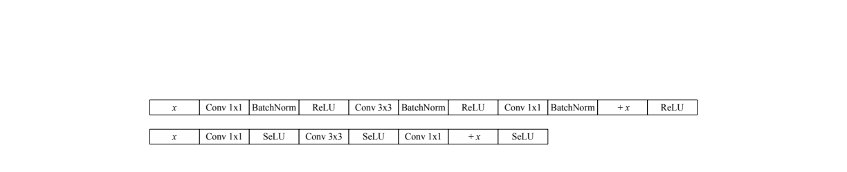
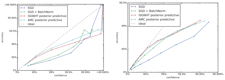
The paper claims that ATMC constructs a stochastic differential equation whose stationary distribution is the posterior over network weights, and simulates it with a split integrator. The central device is a per-parameter temperature variable that adapts the injected noise and momentum damping, so the sampler can compensate for stochastic gradient noise without knowing its covariance. With a ResNet++ architecture that removes BatchNorm and uses SELU activations, Fixup initialization, and weight normalization, the sampler scales to ImageNet: a single posterior sample reaches 74.2% top-1 accuracy, and the posterior predictive reaches 77.5% top-1 accuracy with a test log-likelihood of 0.883 nats, outperforming the SGD-with-BatchNorm baseline at 76.2% and 0.947 nats. The paper further claims that the posterior predictive is nearly perfectly calibrated for low-confidence predictions, unlike the optimization baseline.
Load-bearing premise
The entire posterior-sampling claim rests on the assumption that mini-batch gradient noise is Gaussian with constant, diagonal covariance, so that a single per-parameter thermostat can correct it; the authors themselves state this will not hold in practice and will bias the samples, and the printed integrator exponentials have the opposite friction sign from the SDE.
Editorial extensions
If this is right
- Stochastic-gradient MCMC no longer needs an annealed step size to be useful at scale; a fixed cyclic step size suffices, as used in ATMC.
- A single posterior sample can outperform a well-tuned optimization baseline in a BatchNorm-free architecture, so the cost of Bayesian inference can be as low as one forward pass at test time.
- Averaging posterior samples gives better-calibrated uncertainty estimates, particularly for low-confidence predictions, which matters for decision-making and risk-sensitive applications.
- Because ATMC does not use BatchNorm or Dropout, it opens the way to Bayesian training of vision models without batch statistics, and the paper suggests that the inductive bias of BatchNorm might eventually be encoded as an explicit prior.
- The sampler's robustness to overfitting removes the need for early stopping and careful learning-rate decay schedules in the tested settings.
Reading between the lines
- If the constant-diagonal-covariance assumption on mini-batch gradient noise is violated, ATMC's samples will be biased; a testable prediction is that calibration degrades on tasks where gradient noise is strongly non-Gaussian or highly anisotropic.
- The printed integrator exponentials use e^{+βh} while the SDE in Eq. (4) implies e^{-βh}; if the printed algorithm was actually run, the published numbers may reflect a different friction sign, and re-running with the corrected sign would clarify the discrepancy.
- The same adaptive-thermostat construction could be transferred to other SG-MCMC targets such as variational inference or reinforcement learning, where posterior uncertainty drives exploration.
- Since the sampler ran about 10x longer than the optimization baseline before matching its accuracy, the practical bottleneck is wall-clock time, not final accuracy; ensembling or distillation of the posterior predictive into a single network could narrow that gap.
Signed reviews
Editorial analysis
A structured set of objections, weighed in public.
Referee Report
Summary. The paper introduces ATMC (Adaptive Thermostat Monte Carlo), a stochastic-gradient MCMC method intended to sample from the posterior distribution of a deep neural network. The sampler is derived within the complete-recipe framework of Ma et al. by adding a per-parameter thermostat variable that adaptively controls momentum noise and friction. The authors then construct a second-order Strang-splitting integrator, define a BatchNorm-free ResNet++ architecture using SELU, Fixup initialization, and weight normalization, and report experiments on CIFAR-10 and ImageNet. They claim that a single ATMC sample beats a well-tuned SGD baseline without BatchNorm and that the ATMC posterior predictive beats an SGD baseline with BatchNorm on ImageNet in both accuracy and test log-likelihood, with better calibration. The paper also states explicit caveats: the constant-diagonal covariance assumption on minibatch gradient noise is acknowledged to be false in practice, and the resulting bias is not measured.
Significance. If the central claims held, this would be a significant advance: it would be the first demonstration that an SG-MCMC method can scale to ImageNet-sized problems and outperform a strong optimization baseline on accuracy, log-likelihood, and calibration. The manuscript has several commendable features: it builds on a principled SDE framework, gives a detailed description of hyperparameters, reports both accuracy and NLL, includes calibration plots, and explicitly acknowledges the main modeling approximation. However, the significance is currently undermined by an internal inconsistency between the stated SDE and the printed integrator, together with the unquantified admitted bias. These issues must be resolved before the empirical results can be interpreted as evidence about posterior sampling.
major comments (3)
- [Sec. 3, Eq. (10) and Algorithm 1] The printed integrator does not solve the SDE in Eq. (4). For fixed ξ, Eq. (4) gives dp = −∇L̃(θ)dt − β(ξ)p dt + sqrt(2α(ξ)m)dW, an Ornstein–Uhlenbeck process with friction coefficient β. Its exact update is p_{t+h} = e^{−βh}p_t − (1−e^{−βh})/β ∇L̃(θ_t) + sqrt(m(1−e^{−2βh})/(2β)) η, with negative exponents. Instead, Eq. (10) and Algorithm 1 use e^{+βh}, γ1=(e^{βh}−1)/β, and γ2=(e^{2βh}−1)/β, which are the updates for anti-damped dynamics with +βp. Since β(ξ)=α(ξ)+ξ≥D>0, e^{+βh}>1, so the momentum is amplified at every step. As written, the algorithm cannot converge to the stationary distribution of Eq. (4). The noise prefactor also omits the factor sqrt(m) required by sqrt(2αm)dW. This is a load-bearing inconsistency: the claimed connection between Algorithm 1 and the posterior p(θ|x) is broken as printed.
- [Sec. 2.3 and Sec. 5] The paper explicitly states that the constant-diagonal-covariance assumption for the minibatch gradient noise 'will not hold in practise' and that the approximation will lead to bias in the samples, yet the experiments interpret ATMC outputs as posterior samples and use their calibration as evidence of uncertainty quality. No diagnostic is provided to quantify the resulting bias, no convergence check is reported, and no Monte Carlo standard errors are given for the reported posterior-predictive numbers. Because the central claim is that ATMC samples from the true posterior, the manuscript needs at least a quantitative bias assessment or a comparison against a method with known invariant distribution, and diagnostics showing that the chain actually reaches a stationary regime before sampling begins.
- [Algorithm 1 and Eq. (9)] The thermostat update in Algorithm 1 is inconsistent with Eq. (9). Eq. (9) specifies ξ_{t+h}=ξ_t + h[p_t^2/m − 1], but Algorithm 1 line 11 sets ξ_{t+h}←h[p_{t+h}^2/m − 1], dropping the current ξ_t. Also, Eq. (9) uses p_t for both θ and ξ updates, whereas Algorithm 1 uses p_{t+h} after the momentum update; this changes the splitting order. These discrepancies mean that the pseudocode does not implement the Strang splitting φ_h = φ_{h/2}^B ∘ φ_h^A ∘ φ_{h/2}^B described in Sec. 3, and they make the printed algorithm non-reproducible.
minor comments (5)
- [Figures 2 and 3] The figure legends mention 'iSGNHT' and 'AMC', while the text and tables use 'SGNHT' and 'ATMC'; these labels should be made consistent.
- [Eq. (6)] The norm notation in Eq. (6) is malformed: \|\|\|\|p/M(p)\|\|\|\| should be a single norm, and the expression should be written cleanly to avoid confusion.
- [Sec. 5.1 and 5.2] The benchmark name is spelled inconsistently as 'Cifar10' and 'CIFAR-10'; please use one standard spelling throughout.
- [Sec. 2.4] The phrase 'we find that it can cause exploding momentum variables' is informal; if this is an empirical observation, a reference or a brief explanation of the mechanism would be helpful.
- [Sec. 7] The claim 'we are the first to successfully train neural networks using MCMC on ImageNet' should be supported by an explicit comparison with prior large-scale SG-MCMC work rather than stated without qualification.
Circularity Check
No significant circularity: ATMC's SDE construction, integrator, and experimental claims are self-contained or grounded in external cited work; no prediction reduces to a fitted input.
full rationale
The paper's derivation chain is not circular. The ATMC sampler is constructed by instantiating the general complete-recipe SDE framework of Ma et al. [12] with a specific energy function, noise matrix D, and skew-symmetric matrix Q; the SDE in Eq. (4) is obtained by substitution, and the claimed stationary distribution is inherited from the cited framework rather than assumed from the experimental results. The adaptive thermostat choice α(ξ)=max(D−ξ,0) is presented as an explicit design choice based on avoiding negative friction and is not fitted to the reported accuracies or likelihoods. The numerical integrator in Sec. 3 follows the Strang-splitting and exact Ornstein–Uhlenbeck updates of prior integrator work [15]; its form is derived from the split SDE in Eq. (7), not from the benchmark numbers. The hyperparameters h0, m, c, and D are given interpretable roles (e.g., controlling average and maximum update magnitudes) and are chosen before reporting test performance; they are not fit to make the posterior predictive match a known answer. The empirical claims—accuracy, log-likelihood, calibration—are evaluated on held-out Cifar10 and ImageNet data against external baselines, so the results are not forced by construction. The acknowledged approximation that the stochastic-gradient covariance B is constant and diagonal is a stated bias assumption, and the apparent sign inconsistency in Eq. (10) versus Eq. (4) is an internal correctness concern, not a circularity: neither makes a prediction identical to an input by definition. No load-bearing self-citations or author-imported uniqueness theorems appear; the cited prior works are by other authors and provide independent methodological scaffolding. Therefore the circularity score is 0.
Assumptions & free parameters
free parameters (6)
- Step size h0 =
0.001 (Cifar10), 0.0005 (ImageNet)
- Momentum noise D =
-log(0.9)/h0
- Momentum mass m and speed limit c =
m=(0.0003/h0)^-2, c=0.001/h0
- Cycle length n =
50 epochs (Cifar10), 20 epochs (ImageNet)
- Laplace prior scale b =
5
- Burn-in and sample collection start =
150 epochs
assumptions (4)
- standard math SDE framework of Ma et al. (2015): SDEs of the form in Eq. (1) have p(z) as invariant distribution.
- domain assumption Stochastic gradient noise is Gaussian with diagonal, constant covariance B.
- ad hoc to paper The thermostat choice alpha(xi)=max(D-xi,0) preserves the target invariant distribution.
- domain assumption Beta(p,xi) is held constant in p for the hyperbolic momentum distribution during integration.
Cite this review
Pith. "Pith review of Bayesian Inference for Large Scale Image Classification." pith.science (2026). https://pith.science/paper/JLF3ILC7
@misc{pith2026190803491,
  author       = {Pith},
  title        = {Pith review of: Bayesian Inference for Large Scale Image Classification},
  year         = {2026},
  howpublished = {\url{https://pith.science/paper/JLF3ILC7}},
  note         = {Machine review of arXiv:1908.03491}
}
read the original abstract
Bayesian inference promises to ground and improve the performance of deep neural networks. It promises to be robust to overfitting, to simplify the training procedure and the space of hyperparameters, and to provide a calibrated measure of uncertainty that can enhance decision making, agent exploration and prediction fairness. Markov Chain Monte Carlo (MCMC) methods enable Bayesian inference by generating samples from the posterior distribution over model parameters. Despite the theoretical advantages of Bayesian inference and the similarity between MCMC and optimization methods, the performance of sampling methods has so far lagged behind optimization methods for large scale deep learning tasks. We aim to fill this gap and introduce ATMC, an adaptive noise MCMC algorithm that estimates and is able to sample from the posterior of a neural network. ATMC dynamically adjusts the amount of momentum and noise applied to each parameter update in order to compensate for the use of stochastic gradients. We use a ResNet architecture without batch normalization to test ATMC on the Cifar10 benchmark and the large scale ImageNet benchmark and show that, despite the absence of batch normalization, ATMC outperforms a strong optimization baseline in terms of both classification accuracy and test log-likelihood. We show that ATMC is intrinsically robust to overfitting on the training data and that ATMC provides a better calibrated measure of uncertainty compared to the optimization baseline.
Figures
Forward citations
Cited by 1 Pith paper
-
Stochastic Weight Sharing for Bayesian Neural Networks
2DGBNN compresses Bayesian neural networks by clustering weight means and variances into shared 2D Gaussians, reducing parameter counts by up to 99% on ImageNet-scale models with small accuracy losses.
Reference graph
Works this paper leans on
-
[1]
Alex Kendall and Yarin Gal. What uncertainties do we need in bayesian deep learning for computer vision? In Advances in neural information processing systems , pages 5574–5584, 2017
work page 2017
-
[2]
Privacy for free: Posterior sampling and stochastic gradient monte carlo
Yu-Xiang Wang, Stephen Fienberg, and Alex Smola. Privacy for free: Posterior sampling and stochastic gradient monte carlo. In International Conference on Machine Learning, pages 2493–2502, 2015
work page 2015
-
[3]
Ian Osband and Benjamin Van Roy. Why is posterior sampling better than optimism for reinforcement learning? In Proceedings of the 34th International Conference on Machine Learning-Volume 70, pages 2701–2710. JMLR. org, 2017
work page 2017
-
[4]
Bala Rajaratnam and Doug Sparks. Mcmc-based inference in the era of big data: A funda- mental analysis of the convergence complexity of high-dimensional chains. arXiv preprint arXiv:1508.00947, 2015
arXiv 2015
-
[5]
Bayesian learning via stochastic gradient langevin dynamics
Max Welling and Yee W Teh. Bayesian learning via stochastic gradient langevin dynamics. In Proceedings of the 28th international conference on machine learning (ICML-11) , pages 681–688, 2011
2011
-
[6]
Bayesian posterior sampling via stochastic gradient fisher scoring
Sungjin Ahn, Anoop Korattikara, and Max Welling. Bayesian posterior sampling via stochastic gradient fisher scoring. arXiv preprint arXiv:1206.6380, 2012
arXiv 2012
-
[7]
Bayesian sampling using stochastic gradient thermostats
Nan Ding, Youhan Fang, Ryan Babbush, Changyou Chen, Robert D Skeel, and Hartmut Neven. Bayesian sampling using stochastic gradient thermostats. In Z. Ghahramani, M. Welling, C. Cortes, N. D. Lawrence, and K. Q. Weinberger, editors, Advances in Neural Information Processing Systems 27, pages 3203–3211. Curran Associates, Inc., 2014
work page 2014
-
[8]
Deep residual learning for image recognition
Kaiming He, Xiangyu Zhang, Shaoqing Ren, and Jian Sun. Deep residual learning for image recognition. In Proceedings of the IEEE conference on computer vision and pattern recogni- tion, pages 770–778, 2016
2016
Show all 26 references
-
[9]
Self- normalizing neural networks
G ¨unter Klambauer, Thomas Unterthiner, Andreas Mayr, and Sepp Hochreiter. Self- normalizing neural networks. In Advances in neural information processing systems , pages 971–980, 2017
2017
-
[10]
Fixup initialization: Residual learning without normalization
Hongyi Zhang, Yann N Dauphin, and Tengyu Ma. Fixup initialization: Residual learning without normalization. arXiv preprint arXiv:1901.09321, 2019
1901 arXiv
-
[11]
Weight normalization: A simple reparameterization to accelerate training of deep neural networks
Tim Salimans and Durk P Kingma. Weight normalization: A simple reparameterization to accelerate training of deep neural networks. In Advances in Neural Information Processing Systems, pages 901–909, 2016
2016
-
[12]
A complete recipe for stochastic gradient mcmc
Yi-An Ma, Tianqi Chen, and Emily Fox. A complete recipe for stochastic gradient mcmc. In C. Cortes, N. D. Lawrence, D. D. Lee, M. Sugiyama, and R. Garnett, editors, Advances in Neural Information Processing Systems 28, pages 2917–2925. Curran Associates, Inc., 2015
2015
-
[13]
Stochastic gradient hamiltonian monte carlo
Tianqi Chen, Emily Fox, and Carlos Guestrin. Stochastic gradient hamiltonian monte carlo. In International conference on machine learning, pages 1683–1691, 2014
2014
-
[14]
Relativistic monte carlo
Xiaoyu Lu, Valerio Perrone, Leonard Hasenclever, Yee Whye Teh, and Sebastian J V ollmer. Relativistic monte carlo. arXiv preprint arXiv:1609.04388, 2016. 9
2016 arXiv
-
[15]
On the convergence of stochastic gradient mcmc algorithms with high-order integrators
Changyou Chen, Nan Ding, and Lawrence Carin. On the convergence of stochastic gradient mcmc algorithms with high-order integrators. In Advances in Neural Information Processing Systems, 2015
2015
-
[16]
Dropout: a simple way to prevent neural networks from overfitting
Nitish Srivastava, Geoffrey Hinton, Alex Krizhevsky, Ilya Sutskever, and Ruslan Salakhut- dinov. Dropout: a simple way to prevent neural networks from overfitting. The Journal of Machine Learning Research, 15(1):1929–1958, 2014
1929
-
[17]
Batch normalization: Accelerating deep network training by reducing internal covariate shift
Sergey Ioffe and Christian Szegedy. Batch normalization: Accelerating deep network training by reducing internal covariate shift. In International Conference on Machine Learning, pages 448–456, 2015
2015
-
[18]
Variational dropout and the local reparam- eterization trick
Durk P Kingma, Tim Salimans, and Max Welling. Variational dropout and the local reparam- eterization trick. In Advances in Neural Information Processing Systems , pages 2575–2583, 2015
2015
-
[19]
Bayesian uncertainty estimation for batch normalized deep networks
Mattias Teye, Hossein Azizpour, and Kevin Smith. Bayesian uncertainty estimation for batch normalized deep networks. arXiv preprint arXiv:1802.06455, 2018
2018 arXiv
-
[20]
Wngrad: learn the learning rate in gradient descent
Xiaoxia Wu, Rachel Ward, and L ´eon Bottou. Wngrad: learn the learning rate in gradient descent. arXiv preprint arXiv:1803.02865, 2018
2018 arXiv
-
[21]
Cycli- cal stochastic gradient mcmc for bayesian deep learning
Ruqi Zhang, Chunyuan Li, Jianyi Zhang, Changyou Chen, and Andrew Gordon Wilson. Cycli- cal stochastic gradient mcmc for bayesian deep learning. arXiv preprint arXiv:1902.03932 , 2019
1902 arXiv
-
[22]
Weight uncer- tainty in neural network
Charles Blundell, Julien Cornebise, Koray Kavukcuoglu, and Daan Wierstra. Weight uncer- tainty in neural network. InInternational Conference on Machine Learning, pages 1613–1622, 2015
2015
-
[23]
A simple baseline for bayesian uncertainty in deep learning.arXiv preprint arXiv:1902.02476, 2019
Wesley Maddox, Timur Garipov, Pavel Izmailov, Dmitry Vetrov, and Andrew Gordon Wilson. A simple baseline for bayesian uncertainty in deep learning.arXiv preprint arXiv:1902.02476, 2019
1902 arXiv
-
[24]
Bayesian dark knowledge
Anoop Korattikara Balan, Vivek Rathod, Kevin P Murphy, and Max Welling. Bayesian dark knowledge. In Advances in Neural Information Processing Systems, pages 3438–3446, 2015
2015
-
[25]
Preconditioned stochas- tic gradient langevin dynamics for deep neural networks
Chunyuan Li, Changyou Chen, David Carlson, and Lawrence Carin. Preconditioned stochas- tic gradient langevin dynamics for deep neural networks. In Thirtieth AAAI Conference on Artificial Intelligence, 2016
2016
-
[26]
Stochastic gradient descent as ap- proximate bayesian inference
Stephan Mandt, Matthew D Hoffman, and David M Blei. Stochastic gradient descent as ap- proximate bayesian inference. The Journal of Machine Learning Research, 18(1):4873–4907, 2017. 10
2017
Reviewed August 14, 2026 · model on record in the stance chip above.
Discussion (0). Continue with ORCID to comment.