REVIEW 3 major objections 5 minor 29 references
Chaotic Time Series Prediction using Spatio-Temporal RBF Neural Networks
T0 review · 3 major / 5 minor · reviewed 2026-08-14 · deepseek-v4-flash
Pith's one-line read The proposed spatio-temporal RBF network beats the standard RBF by 5.5 dB in mean squared error on chaotic time series prediction.
desk verdict A clear but unsupported claim of a spatio-temporal RBF; Eq. (5) is a reindexed standard RBF and the comparison uses unmatched hyperparameters. read the letter →
The pith
A machine-rendered reading of the paper's core claim, the machinery that carries it, and where it could break.
The reading
What carries the argument
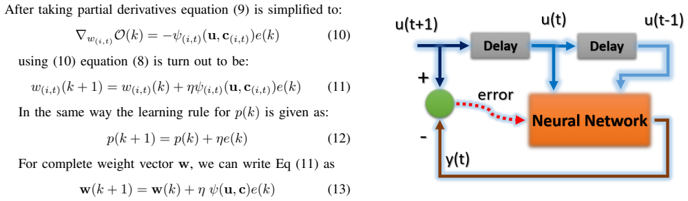
The central object is the spatio-temporal RBF neural network (STRBF-NN) defined by Eq. (5): $$y(k) = \sum_{i=1}^{S} \sum_{t=1}^{T} w_{(i,t)}(k) \psi_{(i,t)}(u, c_{(i,t)}) + p(k)$$ where each hidden unit is indexed by a spatial index $i$ and a temporal index $t$, with its own Gaussian kernel $\psi_{(i,t)}$ and center $c_{(i,t)}$. The double sum is meant to exploit time-space orthogonality by separating the temporal dynamics (indexed by $t$) from the spatial nonlinearity (indexed by $i$). The accompanying gradient-descent weight update, Eq. (11), $w_{(i,t)}(k+1) = w_{(i,t)}(k) + \eta \psi_{(i,t)}(u, c_{(i,t)}) e(k)$, is the mechanism that trains these coupled weights.
What would settle it
Run both networks on the same Mackey-Glass data with identical learning rate and identical Gaussian spread; if the STRBF-NN no longer beats the standard RBF by a few decibels, the reported advantage is a hyperparameter artifact rather than an architectural improvement.
Extended reading notes
Core claim
On its own terms, the paper's central claim is that extending the RBF output from a single sum over spatial neurons to a double sum over spatial and temporal indices—each term having its own Gaussian kernel and weight—enables the network to handle the temporal dynamics and spatial complexity of a chaotic series separately. Trained with gradient descent, this spatio-temporal RBF achieves a mean test MSE of -26.34 dB on the Mackey-Glass series, outperforming the conventional RBF's -20.88 dB. The authors attribute the improvement to the time-space orthogonality that the double-sum structure imposes.
Load-bearing premise
The central claim rests on the assumption that the two-index summation really separates temporal and spatial information, and that the unequal learning rates and kernel widths still make the comparison a fair test of architectural gain.
Editorial extensions
If this is right
- Any existing RBF-based predictor could be restructured with a temporal summation axis, potentially gaining multi-decibel accuracy on chaotic benchmarks without adding neurons.
- The separation of temporal and spatial processing may generalize to other nonlinear time series, such as physiological or financial data, where short history matters.
- The simple gradient update rule makes the method easy to implement on top of standard RBF toolkits.
- The authors' suggestion to replace gradient descent with fractional or q-gradient methods implies that the architecture's accuracy could be pushed further with more sophisticated learning rules.
Reading between the lines
- Because the paper sets the STRBF learning rate five times larger and the kernel spread half that of the standard RBF, a strictly matched hyperparameter comparison would be needed to confirm that the architecture, not the tuning, drives the gain.
- Mathematically, Eq. (5) may be equivalent to a standard RBF with $S \times T$ hidden units if the temporal index is folded into the input vector; checking this equivalence would clarify whether the spatio-temporal description is substantive or notational.
- If the improvement persists across other chaotic systems (e.g., Lorenz or Rössler), the method would be a ready-made upgrade for embedded forecasting applications.
Signed reviews
Editorial analysis
A structured set of objections, weighed in public.
Referee Report
Summary. The paper proposes a spatio-temporal extension of RBF neural networks (STRBF-NN) for chaotic time series prediction. The proposed model, defined in Eq. (5), replaces the single sum over hidden units in a conventional RBF with a double sum over indices i and t, and a gradient-descent weight update rule is derived. The method is tested on the Mackey-Glass time series with 100 Monte Carlo runs, and the authors report a mean testing MSE of -26.34 dB for STRBF-NN versus -20.88 dB for a conventional RBF-NN, concluding that the spatio-temporal architecture significantly improves prediction.
Significance. If the proposed architecture genuinely captured temporal dynamics separately from spatial nonlinearity, it would offer a simple, low-complexity improvement for nonlinear time series forecasting. The manuscript has some strengths: the gradient-descent algebra in Section II is straightforward and correct, the authors report 100 Monte Carlo simulations, and they state that code is available online. However, the central architectural claim is not supported by the manuscript's own equations: Eq. (5) is formally a conventional RBF with S x T hidden units evaluated on the same input vector, and no temporal operator or definition of time-space orthogonality is given. The empirical comparison also uses unequal learning rates and kernel widths without justification, and no error bars are reported. The claimed performance gain therefore cannot be attributed to the proposed architecture, and the paper's main contribution is not established.
major comments (3)
- [Section II, Eq. (5)] The proposed output mapping y(k) = sum_{i=1}^S sum_{t=1}^T w_{i,t}(k) psi_{i,t}(u, c_{i,t}) + p(k) is mathematically identical to a conventional RBF with M = S x T hidden neurons, because every basis function is evaluated at the same input u(k) and the index t appears only as a second summation index. No time delay, recurrent connection, temporal filter, or other time-domain operator is introduced. The manuscript's claims of a 'temporal expansion of signal in kernel space' and 'time-space orthogonality' are never given mathematical definitions. This is a load-bearing issue because it directly undermines the paper's claim to propose a new spatio-temporal architecture.
- [Section III] The experimental comparison does not isolate the effect of the proposed architecture. The conventional RBF uses a learning rate of eta = 1e-2, while the STRBF uses eta = 5e-2, a five-fold difference, and the text states that 'the learning rate and standard deviation of the Gaussian kernel for the proposed STRBF is kept half'—yet the learning rate is five times larger, not half. Since the STRBF of Eq. (5) is a reindexed RBF, the reported 5.46 dB improvement could be entirely due to the larger learning rate, the different kernel widths, or random initialization, rather than to any architectural advantage. Without matched hyperparameters or an ablation, the performance claim loses its stated meaning.
- [Section III, Table I and Fig. 5] The central quantitative claim—that STRBF-NN achieves -26.34 dB versus -20.88 dB for RBF-NN—is reported as a mean over 100 Monte Carlo runs, but no confidence intervals, standard deviations, or error bars are provided. The text gives no indication of the variance across runs, so the reported mean difference is not shown to be statistically significant. Given that this comparison is the paper's main evidence, the lack of uncertainty quantification is a substantive omission.
minor comments (5)
- [Abstract and Section I] There are grammatical errors, including 'difficult predict' and 'an spatio-temporal', which should be corrected ('difficult to predict', 'a spatio-temporal').
- [Section II] The term 'spatio-Temporal' is capitalized inconsistently ('spatio-temporal' appears elsewhere); please use a consistent capitalization convention throughout.
- [Section III] The paper states that the input is 'two samples (one current value and one previous instance value)' and the target is 'a very next future value', but the conclusion says 'two step forward signal of Mackey-Glass time-series is predicted'; these descriptions should be reconciled.
- [References] Some references appear to be mis-cited or duplicated: for example, [8] and [10] are the same reference, and [22] (peri-saccadic perception) does not clearly support the statement about 'estimation of spatio-temporal neural activity using RBF networks'. Please verify all citations.
- [Section II, Fig. 1] Figure 1 is referenced as showing the signal flow of the spatio-temporal RBF, but the text does not describe its contents, and the equations do not reflect the 'parallel temporal layers' mentioned in Section III. Clarify the relationship between the figure and the formal model.
Circularity Check
Eq. (5) reduces to a conventional RBF with S×T hidden units; the 'spatio-temporal' extension is a reindexing, so the central performance claim is not architecturally supported.
-
renaming known result
[Section II, 'Gradient descent-based spatio-Temporal RBFNN', Eq. (5)]
"However in spatio-temporal processing of signal we also need temporal expansion of signal in kernel space as shown in Fig.1. ... y(k) = \sum_{i=1}^{S} \sum_{t=1}^{T} w_{(i,t)}(k)\psi_{(i,t)}(u, c_{(i,t)}) + p(k) (5)"
In Eq. (5), every basis function is evaluated on the same input vector u(k); the index t never enters as a delay, time operator, or separate temporal argument. Flattening with m=(i-1)T+t gives exactly the conventional RBF of Eq. (1) with M=S*T hidden units. The advertised 'temporal expansion of signal in kernel space' and 'time-space orthogonality' are never defined by an operator or equation. Therefore the proposed STRBF is, by construction, a reindexed standard RBF, and the reported validation gain cannot be attributed to a spatio-temporal mechanism.
full rationale
The core reduction is definitional/renaming rather than fit-to-target. The Mackey-Glass benchmark is external and the gradient-descent update is standard, so there is no fitted-parameter circularity in the usual sense. However, the paper's own Eq. (5) is the entire statement of the proposed architecture, and it is formally identical to Eq. (1) after flattening the double sum; t is only a dummy index. The text's 'temporal expansion' and 'time-space orthogonality' are asserted without mathematical content, so the claimed advantage is not derived from a spatio-temporal construction. The comparison in Section III uses unequal hyperparameters (eta=0.01 for RBF versus eta=0.05 for STRBF, sigma kept 'half'), so the 5.46 dB gap is at most a hyperparameter/initialization effect, and no confidence intervals are reported. The many same-group references are background for adaptive and fractional-gradient algorithms and are not load-bearing for the central architecture claim, so they do not add separate circularity.
Assumptions & free parameters
free parameters (4)
- Learning rate for RBF =
1e-2
- Learning rate for STRBF =
5e-2
- Gaussian kernel width ratio =
sigma_STRBF = 0.5 * sigma_RBF
- Hidden unit partition =
20 for RBF; 10+10 for STRBF
assumptions (4)
- standard math Gradient descent chain rule and squared-error objective are valid for training RBF networks.
- domain assumption Mackey-Glass with tau=20, a=0.2, b=0.1 is a representative chaotic time series prediction benchmark.
- ad hoc to paper Time-space orthogonality allows temporal dynamics and spatial nonlinearity to be captured by parallel RBF layers.
- ad hoc to paper Comparing RBF and STRBF under different learning rates and kernel widths isolates the architectural effect.
Cite this review
Pith. "Pith review of Chaotic Time Series Prediction using Spatio-Temporal RBF Neural Networks." pith.science (2026). https://pith.science/paper/JODLH6FZ
@misc{pith2026190808389,
  author       = {Pith},
  title        = {Pith review of: Chaotic Time Series Prediction using Spatio-Temporal RBF Neural Networks},
  year         = {2026},
  howpublished = {\url{https://pith.science/paper/JODLH6FZ}},
  note         = {Machine review of arXiv:1908.08389}
}
read the original abstract
Due to the dynamic nature, chaotic time series are difficult predict. In conventional signal processing approaches signals are treated either in time or in space domain only. Spatio-temporal analysis of signal provides more advantages over conventional uni-dimensional approaches by harnessing the information from both the temporal and spatial domains. Herein, we propose an spatio-temporal extension of RBF neural networks for the prediction of chaotic time series. The proposed algorithm utilizes the concept of time-space orthogonality and separately deals with the temporal dynamics and spatial non-linearity(complexity) of the chaotic series. The proposed RBF architecture is explored for the prediction of Mackey-Glass time series and results are compared with the standard RBF. The spatio-temporal RBF is shown to out perform the standard RBFNN by achieving significantly reduced estimation error.
Figures


Figures from the paper (2 more)


Reference graph
Works this paper leans on
-
[1]
S. Khan, I. Naseem, R. Togneri, and M. Bennamoun, “Rafp-pred: Robust prediction of antifreeze proteins using localized analysis of n-peptide compositions,” IEEE/ACM Transactions on Computational Biology and Bioinformatics, vol. PP, no. 99, pp. 1–1, 2017
work page 2017
-
[2]
Ecmsrc: A sparse learning approach for the prediction of extracellular matrix proteins,
I. Naseem, S. Khan, R. Togneri, and M. Bennamoun, “Ecmsrc: A sparse learning approach for the prediction of extracellular matrix proteins,” Current Bioinformatics, vol. 12, no. 4, pp. 361–368, 2017
work page 2017
-
[3]
Efficient b-mode ultrasound image reconstruction from sub-sampled rf data using deep learning,
Y . H. Yoon, S. Khan, J. Huh, J. C. Yeet al., “Efficient b-mode ultrasound image reconstruction from sub-sampled rf data using deep learning,” IEEE transactions on medical imaging , 2018
work page 2018
-
[4]
Neural networks for control of industrial processes,
B. Schurmann, “Neural networks for control of industrial processes,” in IEE Colloquium on Advances in Neural Networks for Control and Systems, May 1994, pp. 5/1–5/3
work page 1994
-
[5]
A mathematical framework for deep learning in elastic source imaging,
J. Yoo, A. Wahab, and J. Ye, “A mathematical framework for deep learning in elastic source imaging,” SIAM Journal on Applied Mathematics, vol. 78, no. 5, pp. 2791–2818, 2018. [Online]. Available: https://doi.org/10.1137/18M1174027
-
[6]
A novel fractional gradient-based learning algorithm for recurrent neural networks,
S. Khan, J. Ahmad, I. Naseem, and M. Moinuddin, “A novel fractional gradient-based learning algorithm for recurrent neural networks,” Cir- cuits, Systems, and Signal Processing , pp. 1–20, 2017
work page 2017
-
[7]
J. Zhao, W. Chen, and W. Xu, “Nonlinear system identification based on radial basis function neural network using improved particle swarm optimization,” in 2009 Fifth International Conference on Natural Com- putation, vol. 2, Aug 2009, pp. 409–413
work page 2009
-
[9]
A novel adaptive kernel for the rbf neural networks,
S. Khan, I. Naseem, R. Togneri, and M. Bennamoun, “A novel adaptive kernel for the rbf neural networks,” Circuits, Systems, and Signal Processing, pp. 1–15, 2016
work page 2016
Show all 29 references
-
[10]
A fractional gradient descent-based rbf neural network,
S. Khan, I. Naseem, M. A. Malik, R. Togneri, and M. Bennamoun, “A fractional gradient descent-based rbf neural network,” Circuits, Systems, and Signal Processing , pp. 1–22, 2018
2018
-
[11]
VP- FLMS: a novel variable power fractional LMS algorithm,
S. Khan, M. Usman, I. Naseem, R. Togneri, and M. Bennamoun, “VP- FLMS: a novel variable power fractional LMS algorithm,” in 2017 Ninth International Conference on Ubiquitous and Future Networks (ICUFN) (ICUFN 2017), Milan, Italy, Jul. 2017
2017
-
[12]
A robust variable step size fractional least mean square (rvss- flms) algorithm,
——, “A robust variable step size fractional least mean square (rvss- flms) algorithm,” in 13th IEEE Colloquium on Signal Processing and its Applications (CSPA 2017) . IEEE, 2017
2017
-
[13]
Rvp- flms : A robust variable power fractional lms algorithm,
J. Ahmad, M. Usman, S. Khan, I. Naseem, and H. J. Syed, “Rvp- flms : A robust variable power fractional lms algorithm,” in 2016 IEEE International Conference on Control System, Computing and Engineering (ICCSCE). IEEE, 2016
2016
-
[14]
Fclms: Fractional complex lms algorithm for complex system identification,
J. Ahmad, S. Khan, M. Usman, I. Naseem, M. Moinuddin, and H. J. Syed, “Fclms: Fractional complex lms algorithm for complex system identification,” in Signal Processing & its Applications (CSPA), 2017 IEEE 13th International Colloquium on . IEEE, 2017, pp. 39–43
2017
-
[15]
Flmf: Fractional least mean fourth algorithm for channel esti- mation in non-gaussian environment,
S. Khan, N. Ahmed, M. A. Malik, I. Naseem, R. Togneri, and M. Ben- namoun, “Flmf: Fractional least mean fourth algorithm for channel esti- mation in non-gaussian environment,” in 2017 International Conference on Information and Communication Technology Convergence (ICTC) , Oct...
2017
-
[16]
Comments on
S. Khan, A. Wahab, I. Naseem, and M. Moinuddin, “Comments on” design of fractional-order variants of complex lms and nlms algorithms for adaptive channel equalization”,” arXiv preprint arXiv:1802.09252 , 2018
2018 arXiv
-
[17]
Comments on
S. Khan, I. Naseem, A. Sadiq, J. Ahmad, and M. Moinuddin, “Comments on” momentum fractional lms for power signal parameter estimation”,” arXiv preprint arXiv:1805.07640 , 2018
2018 arXiv
-
[18]
Comments and corrections comments on“fractional extreme value adaptive training method: Fractional steepest descent approach
A. Wahab and S. Khan, “Comments and corrections comments on“fractional extreme value adaptive training method: Fractional steepest descent approach”,” IEEE transactions on neural networks and learning systems, 2019
2019
-
[19]
An adaptive learning rate for rbfnn using time-domain feedback analysis,
S. S. A. Ali, M. Moinuddin, K. Raza, and S. H. Adil, “An adaptive learning rate for rbfnn using time-domain feedback analysis,” The scientific world journal , vol. 2014, 2014
2014
-
[20]
A Novel Kernel for RBF Based Neural Networks,
W. Aftab, M. Moinuddin, and M. S. Shaikh, “A Novel Kernel for RBF Based Neural Networks,” Abstract and Applied Analysis , vol. 2014, 2014
2014
-
[21]
On the kernel optimization of radial basis function using nelder mead simplex,
A. K. Hassan, M. Moinuddin, U. M. Al-Saggaf, and M. S. Shaikh, “On the kernel optimization of radial basis function using nelder mead simplex,” Arabian Journal for Science and Engineering , vol. 43, no. 6, pp. 2805–2816, 2018
2018
-
[22]
The peri- saccadic perception of objects and space,
F. H. Hamker, M. Zirnsak, D. Calow, and M. Lappe, “The peri- saccadic perception of objects and space,” PLoS Comput Biol , vol. 4, no. 2, pp. e31–e31, Feb 2008, 18282086[pmid]. [Online]. Available: https://www.ncbi.nlm.nih.gov/pubmed/18282086
2008
-
[23]
Learning spatio-temporal information for multi-object tracking,
J. Wei, M. Yang, and F. Liu, “Learning spatio-temporal information for multi-object tracking,” IEEE Access, vol. 5, pp. 3869–3877, 2017
2017
-
[24]
Geometrical and statistical properties of systems of linear inequalities with applications in pattern recognition,
T. M. Cover, “Geometrical and statistical properties of systems of linear inequalities with applications in pattern recognition,” IEEE Transactions on Electronic Computers , vol. EC-14, no. 3, pp. 326–334, June 1965
1965
-
[25]
Haykin, Neural Networks: A Comprehensive Foundation , 2nd ed
S. Haykin, Neural Networks: A Comprehensive Foundation , 2nd ed. Upper Saddle River, NJ, USA: Prentice Hall PTR, 1998
1998
-
[26]
Topological sensitivity based far-field detection of elastic inclusions,
T. Abbas, S. Khan, M. Sajid, A. Wahab, and J. C. Ye, “Topological sensitivity based far-field detection of elastic inclusions,” Results in physics, vol. 8, pp. 442–460, 2018
2018
-
[27]
Mackey-Glass equation,
L. Glass and M. Mackey, “Mackey-Glass equation,” Scholarpedia, vol. 5, no. 3, p. 6908, 2010, revision #91447
2010
-
[28]
En- hanced q-least mean square,
A. Sadiq, S. Khan, I. Naseem, R. Togneri, and M. Bennamoun, “En- hanced q-least mean square,” Circuits, Systems, and Signal Processing , pp. 1–23, 2019
2019
-
[29]
q-lmf: Quantum calculus-based least mean fourth algorithm,
A. Sadiq, M. Usman, S. Khan, I. Naseem, and M. Moinuddin, “q-lmf: Quantum calculus-based least mean fourth algorithm,” arXiv preprint arXiv:1812.02588, 2018
2018 arXiv
-
[30]
S. Khan. Simulation code. Retrieved November 26, 2018. [Online]. Available: https://tinyurl.com/CTS-Pred-STRBF
2018
Reviewed August 14, 2026 · model on record in the stance chip above.
Discussion (0). Continue with ORCID to comment.