REVIEW 4 major objections 6 minor 37 references
LeDiFlow: Learned Distribution-guided Flow Matching to Accelerate Image Generation
T0 review · 4 major / 6 minor · reviewed 2026-08-07 · deepseek-v4-flash
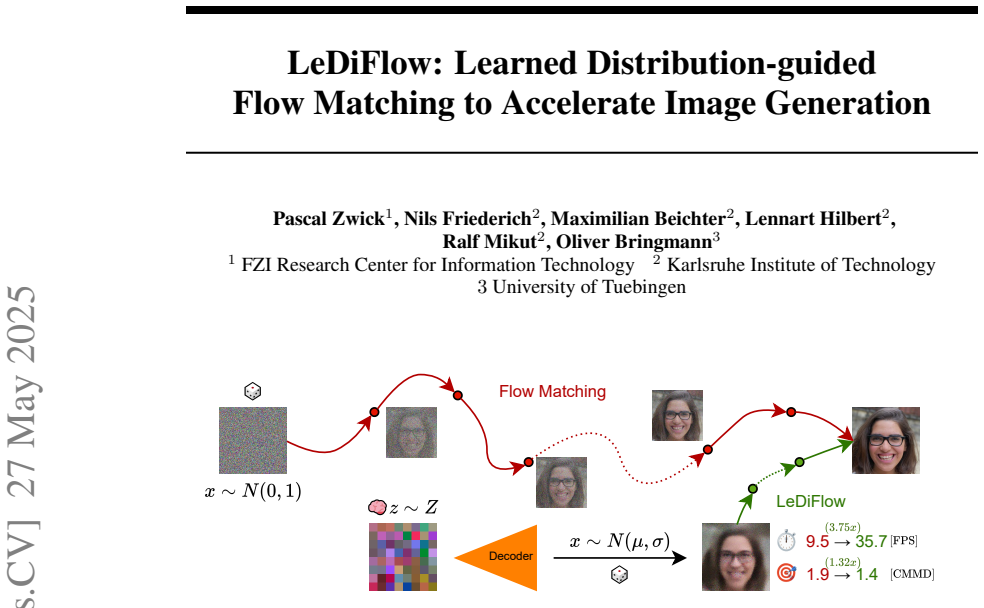
Pith's one-line read Replacing the Gaussian prior with a learned prior makes flow matching need fewer steps, up to 3.75x faster in pixel space and a 1.32x average CMMD gain in latent space.
desk verdict Learned-prior flow matching is a promising idea with a real step-count reduction, but the quality evidence is thinner than the abstract suggests and the sampler-marginal mismatch is a genuine open question. read the letter →
The pith
A machine-rendered reading of the paper's core claim, the machinery that carries it, and where it could break.
The reading
What carries the argument
The load-bearing object is the learned prior $P_L = \mathcal{N}(\mu(z;\theta_D), \sigma^2(z;\theta_D))$ produced by the decoder $\theta_D$ from a latent code $z$, together with the auxiliary encoder-decoder pair that defines the latent space. The decoder is trained with a variance-guided log-likelihood loss, and the flow-matching loss is reweighted per pixel by $1/\sigma(z;\theta_D)$ so confident predictions are refined and uncertain regions are down-weighted. A separate latent sampler $\theta_L$, itself a flow-matching model, maps a Gaussian in latent space to the encoder's latent distribution so that new images can be generated by first sampling $z$, then drawing $x \sim P_L$, and finally integrating the flow field $\theta_{FM}$.
What would settle it
Train or run LeDiFlow with the latent sampler deliberately biased to produce $z$ values far from the encoder's training distribution, for example by adding growing perturbations to $w$ before $\theta_L$ maps it to $z$. If CMMD and FID do not degrade as the bias increases, the claimed benefit of the learned prior is not actually mediated by in-distribution latent sampling; alternatively, if clamping $\sigma(z;\theta_D)$ to a small constant preserves the step-count advantage, the variance prediction is not load-bearing.
Extended reading notes
Core claim
On the paper's own terms, the central discovery is that the prior distribution of a flow-matching model need not be a fixed Gaussian: it can be learned. LeDiFlow trains an auxiliary model to encode each image into a latent vector $z$ and decode that vector into a per-pixel mean and variance, defining a learned prior $P_L = \mathcal{N}(\mu(z;\theta_D), \sigma^2(z;\theta_D))$. Drawing the ODE initial point from this distribution makes the conditional probability path from $x \sim P_L$ to $y \sim Q$ easier to integrate, so a solver with one or two flow steps reaches image quality comparable to or better than the Gaussian-prior baseline with eight steps. The paper demonstrates this on FFHQ, AFHQ, and LHQ, and reports that the latent-space variant improves CMMD on average by a factor of 1.32 while the pixel-space variant speeds up inference by up to 3.75x.
Load-bearing premise
The method assumes that latents drawn by the latent sampler at inference time fall in the same region of the latent space as the encoder outputs used in training, so the decoder's predicted prior and the flow field are evaluated on in-distribution inputs; the KL term encourages, but does not guarantee, that match.
Editorial extensions
If this is right
- A flow-matching generator can trade a fixed Gaussian prior for a cheap learned prior and cut inference steps: pixel-space LeDiFlow reaches baseline quality with up to 3.75x less inference time.
- At one or two flow-matching steps with a second- or third-order ODE solver, LeDiFlow matches or beats the Gaussian-prior baseline at eight steps on FFHQ, AFHQ, and LHQ.
- The learned prior provides conditional control for free: interpolating in the Gaussian latent space and inpainting with a masked vector field produce valid images without retraining.
- The quality gain is not tied to distillation or reflowing; the easier transport comes from the initial distribution itself.
Reading between the lines
- Beyond the reported datasets, the same recipe should apply to any flow-matching model where a cheap conditional predictor can approximate the target: the closer the start distribution, the fewer integration steps, so the idea could transfer to text-to-image or video models if the auxiliary predictor is scaled.
- The per-image Gaussian prior effectively factors one hard transport into two easier transports, Gaussian to latent and latent-conditioned prior to image; if this factorization is the true source of the speedup, then other factorization schemes, such as hierarchical or multi-scale priors, should show similar gains.
- A testable extension is to combine LeDiFlow with path straightening via reflow: since LeDiFlow attacks the starting distribution and reflow attacks the learned path, their benefits may be additive.
- The paper's plateau in CMMD at higher step counts suggests the learned prior constrains the achievable distribution; measuring diversity at high steps would clarify whether the prior limits variability or the solver's error accumulates.
Editorial analysis
A structured set of objections, weighed in public.
Referee Report
Summary. LeDiFlow proposes to replace the standard Gaussian prior in flow-matching image generation with a learned per-image Gaussian prior PL(z) = N(mu(z; theta_D), sigma^2(z; theta_D)), produced by a VAE-style encoder/decoder auxiliary model. The paper claims this makes the learned flow-matching transport easier, so the ODE solver requires fewer steps and yields faster inference, while preserving or improving image quality. The method is evaluated on FFHQ, AFHQ, LHQ and ImageNet, in both pixel space and the latent space of a Stable Diffusion VAE, comparing against a standard flow-matching baseline with the same HDiT backbone. Reported results include a 3.75x pixel-space inference speedup and an average 1.32x CMMD improvement in the latent setup.
Significance. If the claims hold, the idea of conditioning the flow-matching prior on a learned latent code is a useful contribution to efficient generative modeling, especially since it avoids distillation or reflow. The paper includes a concrete architecture, training losses, and experiments on multiple datasets, and it self-identifies several limitations. The strongest part is the step-count reduction: Table 1 and Figure 3 show that LeDiFlow reaches competitive CMMD with far fewer FM solver calls than the standard baseline. However, the quality claims are only partially supported, and the theoretical premise that PL is close to Q is not demonstrated quantitatively. The method's central mechanism therefore remains plausible but not fully verified.
major comments (4)
- [Table 1 and Section 4.1] The headline 'up to 3.75x faster' claim is not matched by equal quality at the compared step budgets. In pixel space, LeDiFlow's CMMD is worse than FM's on FFHQ (2.66 vs 2.48) and AFHQ (1.33 vs 1.08) when FM uses 8 steps and LeDiFlow uses 4 latent + 2 FM steps. The text says results show 'competitive or superior image quality,' but the table shows LeDiFlow is worse on two of three pixel-space datasets. To support the speedup claim, the comparison should be made at iso-quality (e.g., the number of steps each method needs to reach a fixed CMMD threshold), or the quality metric should be reported for matched step budgets and the discrepancy honestly stated.
- [Section 3.1, Eq. (5)] The central premise that PL is 'closer to the target data distribution' is not established. The Variance Guided Loss in Eq. (4) maximizes the conditional log-likelihood log N(y | mu(z), sigma^2(z)) for encoder latents z, not the marginal prior obtained by integrating over z. No experiment measures the distance between the marginal of PL and Q (e.g., FID/CMMD of samples x ~ PL without any flow steps, or an estimate of marginal likelihood). Without such evidence, the claim that the learned prior simplifies the transport problem is a stated assumption rather than a demonstrated property.
- [Section 3.3 and Figure 2] The inference-time z is sampled from the latent flow model theta_L, but theta_D and theta_FM are trained on encoder latents from theta_E. The KL term in Eq. (5) with beta=1e-3 is only a soft regularizer, and the paper provides no evidence that the marginal of theta_L matches the encoder's marginal, nor any statistics on sigma(z; theta_D) (e.g., the fraction of values hitting the 1e-3 clip, histograms, or minimum standard deviations). Section 5 acknowledges the sigma-to-zero risk, but without measurement the observed speedup could be partly due to a near-deterministic decoder emitting image-like starts, rather than to genuinely easier flow paths. Reporting the distributional match of z and the empirical range of sigma is load-bearing for the central claim.
- [Table 1 and Abstract] The '1.32x average improvement' in CMMD for the latent setup is an average over ratios and hides a per-dataset failure: on AFHQ (SDV), LeDiFlow is worse (0.87 vs 0.81), while on FFHQ and ImageNet it is better. The abstract and conclusion claim 'comparable or better' image quality, but the measurements are mixed. The authors should present per-dataset numbers and avoid aggregate statements that obscure negative results.
minor comments (6)
- [Table 1 and References] Dataset citations are swapped: AFHQ is introduced in the StarGAN v2 paper [3], while LHQ is associated with [32] (Skorokhodov et al.). Table 1 and captions of Figures 4 and 12 currently label AFHQ as [32] and LHQ as [3], which will mislead readers.
- [Eq. (6)] The importance-weighted loss is written as ||v_t(...) - (y-x)||^2 1/sigma(z;theta_D), but the operation is ambiguous. Please specify whether the division is element-wise on the squared error and clarify how the clipping to a maximum denominator of 1e-3 is applied (e.g., sigma_clipped = max(sigma, 1e-3)).
- [Section 3.1] Notation is inconsistent: the paper alternates between sigma(z;theta_D) and sigma(z, theta_D), and between mu(z;theta_D) and mu(y;theta_D) in the symbol table (Table 2). Please standardize the notation and ensure it matches the equations.
- [Table 1] The inference-time table footnote states that the SDV decoding cost is approximately 20 ms per image, but the reported times '80' and '40' appear to already include this cost. Please clarify in the table header whether the times include decoding.
- [Figure 3] The caption calls the plots 'Visual scatter plot,' but they are line or marker plots of CMMD versus step count, not scatter plots. Please correct the wording.
- [Section 6] The conclusion says the method needs 'half to one-third of the inference time,' but the abstract reports up to 3.75x, which is less than one-third. Please make the statements consistent and specify the configuration to which each factor applies.
Circularity Check
No substantive circularity: the learned-prior mechanism is trained by maximum likelihood and evaluated against an independent FM baseline on external metrics.
full rationale
The paper's derivation chain is not circular in any definitional or self-citation sense. The learned prior P_L = N(mu(z;theta_D), sigma^2(z;theta_D)) is obtained by optimizing the variance-guided loss in Eq. (4) plus the KL term in Eq. (5) on encoder latents, not by fitting the step-count reduction. The flow-matching model is trained with the conditional importance-weighted loss in Eq. (6) against target images y, and the latent sampler is trained with the standard rectified-flow loss in Eq. (2) on encoder latents. The claimed speedup is then measured on held-out quality metrics (CMMD and FID) in Table 1 and Figures 3, 8, and 9, comparing LeDiFlow against the same HDiT architecture with a Gaussian prior. No fitted parameter is renamed as a prediction, no load-bearing argument reduces to a self-citation, and no uniqueness theorem is imported from the authors' prior work. The only mild conceptual concern is that a prior learned to be close to the target distribution naturally shortens the transport distance, so part of the speedup is by construction; however, this is the explicitly stated mechanism rather than a circular derivation, and Section 5 openly acknowledges the dependence on prior quality and the sigma-approximately-zero collapse risk. Those are robustness limitations, not circularity. Hence the score is low, reflecting a small flavor of tautology in the design rationale but no circular step in the method or evaluation.
Assumptions & free parameters
free parameters (4)
- beta (VAE KL weight) =
1e-3
- Importance-weight denominator floor =
1e-3
- Inference step budget =
4 latent + 2 FM steps (Midpoint), 2 + 1 steps (Heun3)
- Latent dimension k =
256 (8x8x4)
assumptions (4)
- standard math Conditional flow matching with the rectified flow objective (Eq. 2) yields a valid marginal vector field for the learned prior PL.
- domain assumption The per-pixel Gaussian PL = N(mu(z;theta_D), sigma^2(z;theta_D)) is a useful approximation of the conditional target distribution Q given z.
- domain assumption KL regularization makes the latent space Z sufficiently continuous that a Gaussian-to-Z flow sampler theta_L can generate valid codes.
- ad hoc to paper The clipping of the importance-weight denominator at 1e-3 preserves a well-behaved training signal.
invented entities (1)
-
Learned prior distribution PL = N(mu(z;theta_D), sigma^2(z;theta_D))
Cite this review
Pith. "Pith review of LeDiFlow: Learned Distribution-guided Flow Matching to Accelerate Image Generation." pith.science (2026). https://pith.science/paper/KIME3UTB
@misc{pith2026250520723,
  author       = {Pith},
  title        = {Pith review of: LeDiFlow: Learned Distribution-guided Flow Matching to Accelerate Image Generation},
  year         = {2026},
  howpublished = {\url{https://pith.science/paper/KIME3UTB}},
  note         = {Machine review of arXiv:2505.20723}
}
read the original abstract
Enhancing the efficiency of high-quality image generation using Diffusion Models (DMs) is a significant challenge due to the iterative nature of the process. Flow Matching (FM) is emerging as a powerful generative modeling paradigm based on a simulation-free training objective instead of a score-based one used in DMs. Typical FM approaches rely on a Gaussian distribution prior, which induces curved, conditional probability paths between the prior and target data distribution. These curved paths pose a challenge for the Ordinary Differential Equation (ODE) solver, requiring a large number of inference calls to the flow prediction network. To address this issue, we present Learned Distribution-guided Flow Matching (LeDiFlow), a novel scalable method for training FM-based image generation models using a better-suited prior distribution learned via a regression-based auxiliary model. By initializing the ODE solver with a prior closer to the target data distribution, LeDiFlow enables the learning of more computationally tractable probability paths. These paths directly translate to fewer solver steps needed for high-quality image generation at inference time. Our method utilizes a State-Of-The-Art (SOTA) transformer architecture combined with latent space sampling and can be trained on a consumer workstation. We empirically demonstrate that LeDiFlow remarkably outperforms the respective FM baselines. For instance, when operating directly on pixels, our model accelerates inference by up to 3.75x compared to the corresponding pixel-space baseline. Simultaneously, our latent FM model enhances image quality on average by 1.32x in CLIP Maximum Mean Discrepancy (CMMD) metric against its respective baseline.
Figures


Figures from the paper (9 more)


Reference graph
Works this paper leans on
-
[1]
J. C. Butcher. Coefficients and error bounds for Runge-Kutta methods.Mathematics of Computation, 21(100):637–644, 1967. doi: 10.2307/2004864. URL https://doi.org/10. 2307/2004864
-
[2]
T. Q. Chen, Y . Rubanova, J. Bettencourt, and D. Duvenaud. Neural ordinary differential equations. InAdvances in Neural Information Processing Systems (NeurIPS), pages 6571–6583, 2018
work page 2018
-
[3]
Y . Choi, Y . Uh, J. Yoo, and J.-W. Ha. StarGAN v2: Diverse Image Synthesis for Multiple Domains. InProceedings of the IEEE/CVF Conference on Computer Vision and Pattern Recognition (CVPR), pages 8188–8197, 2020
work page 2020
- [4]
-
[5]
K. Crowson, S. A. Baumann, A. Birch, T. M. Abraham, D. Z. Kaplan, and E. Shippole. Scalable high-resolution pixel-space image synthesis with hourglass diffusion transformers. In 9 Proceedings of the IEEE/CVF Conference on Computer Vision and Pattern Recognition (CVPR), pages 567–576, 2024. doi: 10.48550/arXiv.2401.11605
-
[6]
J. Deng, W. Dong, R. Socher, L.-J. Li, K. Li, and L. Fei-Fei. ImageNet: A large-scale hierarchical image database. InProceedings of the IEEE/CVF Conference on Computer Vision and Pattern Recognition (CVPR), pages 248–255. IEEE, 2009
work page 2009
-
[7]
A. Dosovitskiy, L. Beyer, A. Kolesnikov, D. Weissenborn, X. Zhai, T. Unterthiner, M. Dehghani, M. Minderer, G. Heigold, S. Gelly, J. Uszkoreit, and N. Houlsby. An image is worth 16x16 words: Transformers for image recognition at scale. InInternational Conference on Learning Representations, 2021. URLhttps://arxiv.org/abs/2010.11929
arXiv 2021
-
[8]
P. Esser, R. Rombach, and B. Ommer. Taming transformers for high-resolution image synthesis. InProceedings of the IEEE/CVF Conference on Computer Vision and Pattern Recognition (CVPR), pages 12873–12883, 2021. doi: 10.48550/arXiv.2012.09841
Show all 37 references
-
[9]
Esser, S
P. Esser, S. Kulal, A. Blattmann, R. Entezari, J. Müller, H. Saini, Y . Levi, D. Lorenz, A. Sauer, F. Boesel, et al. Scaling rectified flow transformers for high-resolution image synthesis. In Forty-First International Conference on Machine Learning, 2024
2024
-
[10]
Goodfellow, J
I. Goodfellow, J. Pouget-Abadie, M. Mirza, B. Xu, D. Warde-Farley, S. Ozair, A. Courville, and Y . Bengio. Generative adversarial networks. InAdvances in Neural Information Processing Systems (NeurIPS), pages 2672–2680, 2014
2014
-
[11]
Heusel, H
M. Heusel, H. Ramsauer, T. Unterthiner, B. Nessler, and S. Hochreiter. GANs Trained by a Two Time-Scale Update Rule Converge to a Local Nash Equilibrium. InAdvances in Neural Information Processing Systems (NeurIPS), pages 6626–6637, 2017
2017
-
[12]
Higgins, L
I. Higgins, L. Matthey, A. Pal, C. Burgess, X. Glorot, M. Botvinick, S. Mohamed, and A. Lerchner. Beta-V AE: Learning Basic Visual Concepts with a Constrained Variational Framework. InProceedings of the 5th International Conference on Learning Representations (ICLR), 2017
2017
-
[13]
G. E. Hinton and R. R. Salakhutdinov. Reducing the dimensionality of data with neural networks. Science, 313(5786):504–507, 2006
2006
-
[14]
J. Ho, A. Jain, and P. Abbeel. Denoising diffusion probabilistic models.Advances in Neural Information Processing Systems (NeurIPS), 33:6840–6851, 2020
2020
-
[15]
Hukkelås and F
H. Hukkelås and F. Lindseth. DeepPrivacy2: Towards Realistic Full-Body Anonymization. In Proceedings of the IEEE/CVF Winter Conference on Applications of Computer Vision (WACV), 2023
2023
-
[16]
Jayasumana, S
S. Jayasumana, S. Ramalingam, A. Veit, D. Glasner, A. Chakrabarti, and S. Kumar. Rethinking FID: Towards a Better Evaluation Metric for Image Generation. InProceedings of the IEEE/CVF Conference on Computer Vision and Pattern Recognition (CVPR), pages 1–12, 2023. URL https://a...
2023 arXiv
-
[17]
Karras, S
T. Karras, S. Laine, and T. Aila. Flickr-Faces-HQ Dataset (FFHQ), 2019. URL https: //github.com/NVlabs/ffhq-dataset
2019
-
[18]
Karras, M
T. Karras, M. Aittala, T. Aila, and S. Laine. Elucidating the design space of diffusion-based generative models. InProceedings of the Conference on Neural Information Processing Systems (NeurIPS), 2022. URLhttps://papers.nips.cc/paper/2022/hash/edm.pdf
2022
-
[19]
D. P. Kingma and M. Welling. Auto-Encoding Variational Bayes. InProceedings of the 2nd International Conference on Learning Representations (ICLR), 2014
2014
-
[20]
B. F. Labs. Flux.1: A rectified flow transformer for text-to-image generation. https:// huggingface.co/black-forest-labs/FLUX.1-dev, 2023
2023
-
[21]
S. Lee, B. Kim, and J. C. Ye. Minimizing trajectory curvature of ode-based generative models. InInternational Conference on Machine Learning, pages 18957–18973. PMLR, 2023
2023
-
[22]
J. Li, Y . Xu, T. Lv, L. Cui, C. Zhang, and F. Wei. DiT: Self-supervised Pre-training for Document Image Transformer. InProceedings of the 30th ACM International Conference on Multimedia, pages 2975–2983. ACM, 2022. doi: 10.1145/3503161.3547999
2022
-
[23]
Lipman, R
Y . Lipman, R. T. Chen, H. Ben-Hamu, M. Nickel, and M. Le. Flow matching for generative modeling.arXiv preprint arXiv:2210.02747, 2022. 10
2022 arXiv
-
[24]
K. Liu, W. Tang, F. Zhou, and G. Qiu. Spectral Regularization for Combating Mode Collapse in GANs. InProceedings of the IEEE/CVF International Conference on Computer Vision (ICCV), pages 6382–6390, 2019
2019
-
[25]
X. Liu, C. Gong, and Q. Liu. Flow straight and fast: Learning to generate and transfer data with rectified flow.arXiv preprint arXiv:2209.03003, 2022
2022 arXiv
-
[26]
Nie and A
W. Nie and A. B. Patel. Towards a Better Understanding and Regularization of GAN Training Dynamics. InProceedings of the Conference on Uncertainty in Artificial Intelligence (UAI), pages 91–101, 2019. URLhttp://auai.org/uai2019/proceedings/papers/91.pdf
2019
-
[27]
K. Pearson. On lines and planes of closest fit to systems of points in space.The London, Edinburgh, and Dublin Philosophical Magazine and Journal of Science, 2(11):559–572, 1901. doi: 10.1080/14786440109462720
1901 doi
-
[28]
Preechakul, N
K. Preechakul, N. Chatthee, S. Wizadwongsa, and S. Suwajanakorn. Diffusion autoencoders: Toward a meaningful and decodable representation. InProceedings of the IEEE/CVF Conference on Computer Vision and Pattern Recognition (CVPR), pages 10619–10628, 2022
2022
-
[29]
Rombach, A
R. Rombach, A. Blattmann, D. Lorenz, P. Esser, and B. Ommer. High-Resolution Image Synthesis with Latent Diffusion Models. InProceedings of the IEEE/CVF Conference on Computer Vision and Pattern Recognition (CVPR), pages 10684–10695, 2022
2022
-
[30]
Ronneberger, P
O. Ronneberger, P. Fischer, and T. Brox. U-Net: Convolutional Networks for Biomedical Image Segmentation. InMedical Image Computing and Computer-Assisted Intervention – MICCAI 2015, pages 234–241. Springer, Cham, 2015. doi: 10.1007/978-3-319-24574-4_28
2015 doi
-
[31]
Sauer, D
A. Sauer, D. Lorenz, A. Blattmann, and R. Rombach. Adversarial diffusion distillation. In Proceedings of the IEEE/CVF Conference on Computer Vision and Pattern Recognition (CVPR),
-
[32]
Skorokhodov, G
I. Skorokhodov, G. Sotnikov, and M. Elhoseiny. Aligning latent and image spaces to connect the unconnectable.arXiv preprint arXiv:2104.06954, 2021
2021 arXiv
-
[33]
van den Oord, O
A. van den Oord, O. Vinyals, and K. Kavukcuoglu. Neural Discrete Representation Learning. InProceedings of the Conference on Neural Information Processing Systems (NeurIPS), pages 6306–6315, 2017. URLhttps://arxiv.org/abs/1711.00937
2017 arXiv
-
[34]
Vaswani, N
A. Vaswani, N. Shazeer, N. Parmar, J. Uszkoreit, L. Jones, A. N. Gomez, L. Kaiser, and I. Polosukhin. Attention is all you need. InAdvances in Neural Information Processing Systems (NeurIPS), pages 5998–6008, 2017
2017
-
[35]
Zhang, A
L. Zhang, A. Rao, and M. Agrawala. Adding conditional control to text-to-image diffusion models. InProceedings of the IEEE/CVF International Conference on Computer Vision (ICCV), 2023
2023
-
[36]
Zwick, K
P. Zwick, K. Roesch, M. Klemp, and O. Bringmann. Context-aware full body anonymization using text-to-image diffusion models. InProceedings of the 12th International Workshop on Assistive Computer Vision and Robotics (ACVR) in conjunction with ECCV, 2024. 11 12 Appendix Symbol ...
2024
-
[2024]
URLhttps://arxiv.org/abs/2311.17042
Reviewed August 7, 2026 · model on record in the stance chip above.
Discussion (0). Sign in to comment.