REVIEW 4 major objections 6 minor 22 references
Quantum Geometry of Data
T0 review · 4 major / 6 minor · reviewed 2026-08-06 · deepseek-v4-flash
Pith's one-line read The paper claims that the Hermitian matrices learned by quantum cognition machine learning (QCML) define a quantum geometry, and that reading out its metric, Berry curvature, Chern numbers, and matrix Laplacian spectrum recovers the…
desk verdict A conditional but genuinely interesting demonstration: one strong quantitative check, several suggestive ones, and a load-bearing hyperparameter issue that needs a fix. read the letter →
The pith
A machine-rendered reading of the paper's core claim, the machinery that carries it, and where it could break.
The reading
What carries the argument
The central object is the matrix configuration, a set of Hermitian observables interpreted as quantized coordinate functions on the data manifold. The displacement Hamiltonian assigns to each feature-space point a quasi-coherent ground state, and the loss forces the configuration to approximate the data while controlling quantum fluctuations. Geometry is extracted from the matrix Laplacian, defined as the sum of double commutators of the observables, whose eigenmaps give reduced embeddings, and from the quantum geometric tensor, whose imaginary part is the Berry curvature that integrates to integer Chern numbers around degeneracy points.
What would settle it
Train QCML on a dataset of two well-separated spheres with several values of the fluctuation weight w and several random initializations; if the matrix Laplacian spectrum does not consistently show exactly one near-zero mode per sphere and the monopole charges do not remain ±1 at the expected locations, the claim that QCML learns the underlying quantum geometry would be falsified. A more direct test is to use a manifold of odd dimension, such as a circle or line segment, and check whether the learned Berry curvature and Chern numbers stabilize to the expected degenerate-limit values for any non-commuting configuration.
Extended reading notes
Core claim
The paper establishes that the QCML training procedure, which minimizes a loss combining displacement and quantum fluctuation, produces a matrix configuration whose displacement Hamiltonian's ground states define quasi-coherent states, and the abstract space of these states carries a quantum metric, Berry curvature, and matrix Laplacian spectrum that reproduce the geometry of the data manifold. In the synthetic examples the learned operators are shown to be close to exact fuzzy-sphere generators, the matrix Laplacian spectrum exhibits the degeneracies expected for a sphere, and integer-valued Chern numbers are sourced by degeneracy points (monopoles) of the displacement Hamiltonian. The authors state: 'We demonstrate that, for geometric synthetic datasets, QCML effectively learns the quantum geometry of the corresponding geometric objects.'
Load-bearing premise
The trained matrix configuration actually lands in the almost-commutative semiclassical regime, neither a trivial commuting K-means solution nor a random deep-quantum configuration, so that the extracted quantum-geometric invariants reflect the data manifold rather than artifacts of optimization.
Editorial extensions
If this is right
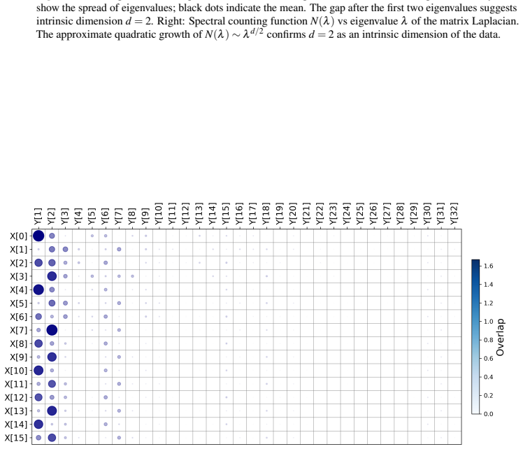
- Intrinsic dimension of a dataset can be read from the spectral gap of the quantum metric or from the Weyl-law slope of the matrix Laplacian counting function, without building neighbor graphs.
- The zero modes and low-lying spectrum of the matrix Laplacian provide a non-graph-based way to detect disconnected components and coarse topology of high-dimensional data.
- Chern numbers computed from learned Berry curvature give integer-valued, deformation-stable topological signatures that can classify datasets or reveal non-contractible loops in data manifolds.
- The eigenmaps of the matrix Laplacian yield a reduced set of matrices that acts as a data-driven analogue of classical Laplacian eigenmaps, compressing the geometry with minimal commutator energy.
- Because geometry is encoded in operator spectra rather than pairwise distances, the representation avoids the curse of dimensionality for data concentrated near low-dimensional manifolds.
Reading between the lines
- The paper leaves open how to choose the fluctuation weight w so that the optimizer reliably lands in the almost-commutative semiclassical regime; a principled criterion or a regularizer that enforces almost-commutativity would make the geometric readout reproducible.
- The even-dimensional nature of symplectic quantum geometry suggests that odd-dimensional manifolds are represented only as degenerate limits, which may limit the accuracy of geometric invariants for such data.
- The degeneracy points and their topological charges could serve as a data-driven clustering or classification signal, since they encode where the Hamiltonian's ground state becomes degenerate and how the Berry curvature is concentrated.
- The framework's claim that learning can be modeled as a topological phase transition is a speculative direction: one could test it by tracking the matrix Laplacian spectrum and Chern numbers during training to see if qualitative jumps coincide with abrupt improvements in generalization.
Editorial analysis
A structured set of objections, weighed in public.
Referee Report
Summary. The paper proposes that the QCML representation—learned Hermitian matrices X_a and quasi-coherent states |x_t⟩ obtained from loss (4)—defines a quantum (fuzzy) geometry whose semiclassical invariants reproduce the geometry of the data manifold. After reviewing quantum geometry, the authors extract the quantum metric, Berry curvature and monopole charges, matrix-Laplacian spectra, and Laplacian eigenmaps for four synthetic examples (uniform sphere, two noisy spheres, non-uniform sphere, conformal maps, with a higher-dimensional Blaschke-Potapov extension) and for the Wisconsin Breast Cancer dataset. The central claim is that global geometric and topological structure—connectivity, intrinsic dimension, Chern numbers—can be read off from operator data rather than from pointwise distances.
Significance. If the claim is correct, the paper introduces a genuinely new operator-based paradigm for manifold learning, with integer topological invariants and spectral dimension estimates that are not fitted to the targets. The quantitative sphere check in Eq. (6) is a genuine falsifiable comparison, and the paper is unusually explicit about failure modes: Section 3 states that w=1 collapses to K-means, and Appendix C distinguishes almost-commutative from deep-quantum configurations. The significance is currently conditional: the semiclassical regime is not certified, the scaling check uses only N=4, and several high-dimensional claims are asserted without shown evidence. With those gaps filled, the paper would be a substantial contribution to the literature on noncommutative geometry in data science.
major comments (4)
- [Section 3, Eq. (4), and Appendix C] The central claim is conditional on the trained configurations lying in the almost-commutative regime, yet no diagnostic is reported that certifies this regime. The paper itself notes in Section 3 that w=1 gives commuting K-means configurations and that "there is no clear principle at the moment for choosing w other than experimentation with the data," and all examples use w=0.1. Please report, for each trained configuration, a normalized commutator ratio such as \|[X_a,X_b]\|_2 / \|X_a X_b\|_2 or the Laplacian energy E(X)/(\lambda_max \|X\|_2^2), together with the number of near-zero Laplacian modes, to show that the configuration is neither a trivial commuting solution nor a deep-quantum random configuration.
- [Section 3 and Figure 4] The only quantitative validation of the fuzzy-sphere geometry uses N=4, the smallest nontrivial case, where the commutator-to-product ratio is of order one and hence does not probe a semiclassical limit. Please add scaling tests at larger N (e.g., N=8, 16, 32) showing that the normalized commutator decreases, that the Laplacian degeneracies approach 2\ell+1, and that the spectrum match is not achieved solely through a free rescaling of the exact fuzzy-sphere spectrum.
- [Section 5.3, after Eq. (29)] The Blaschke-Potapov generalization states that "the intrinsic dimension was correctly computed at all sample points for all tested dimensions" without any figure, table, or error metric. This is a load-bearing claim for the high-dimensional generalization of the method. Please provide the supporting evidence, for example quantum-metric gap plots analogous to Figure 10 or quantitative dimension estimates with uncertainties for n=2,3,4,5.
- [Section 5.4] For the Wisconsin Breast Cancer dataset, the paper asserts that the spectrum "supports an intrinsic dimension of two, consistent with an analysis based on Weyl's law (not shown)" and that Ref. 8 gives an intrinsic-dimension estimate of two, but no Weyl-law plot or quantitative estimate is presented. Since this is the only real-world validation, please include the Weyl-law fit and the intrinsic-dimension estimate, or soften the claim accordingly.
minor comments (6)
- [Section 1] In the sentence "where noa priorigeometric knowledge is available," the spacing around "a priori" is missing.
- [Section 4.3] The matrix Laplacian in Eq. (21) is positive semi-definite rather than positive-definite, since the identity matrix is always a zero mode; the text should be adjusted accordingly.
- [Figure 4] The caption does not specify the horizontal axis or the value of the rescaling factor used for the exact eigenvalues; please state these details.
- [Section 5.1] The claim that the number of monopoles near each sphere (four versus two) "reflects the ratio of their surface areas" is not derived; either provide a derivation or rephrase as an observation.
- [Section 6] The first sentence of the fourth paragraph contains a typo: "there several directions" should be "there are several directions."
- [Appendix D] The table lists noise levels and hyperparameters but no random seeds, initialization scheme, or training details, which makes the numerical results hard to reproduce.
Circularity Check
No significant circularity: geometric invariants are computed from learned matrices and checked against known ground truth, not fitted as targets.
full rationale
The derivation chain is: data X -> optimized Hermitian matrices {X_a} via loss (4) -> quasi-coherent states via the displacement Hamiltonian (1) -> quantum metric and Berry curvature (18), Chern numbers (19), matrix Laplacian (21), and eigenmaps. No reported quantity is fitted to a target: the loss contains only displacement and variance terms, and the geometric outputs are functions of the trained matrices. In the uniform-sphere example the learned matrices are compared with angular-momentum generators after the analytic normalization alpha = 1/(j+w) derived from the same loss; this is a consistency check, and the commutator and Casimir norms are additional content not present in the loss. The intrinsic-dimension estimates in Sections 5.3 and 5.4 use the approach of Ref. [8], which shares authors with this paper, but the synthetic datasets have known ground-truth dimension, so the validation does not depend on the cited work being true; an independent estimator would face the same data. The quantum-geometry formalism is imported from the established mathematical-physics literature (Refs. 12-14, 17) and is not invoked as a uniqueness theorem that forbids alternatives. The admitted hand-tuning of w (Section 3: 'there is no clear principle at the moment for choosing w other than experimentation with the data') and the warning in Section 6 that trained configurations may lie 'far from any semiclassical limit' are correctness and robustness risks, not circularity: they concern whether the learned geometry is meaningful, not whether the derivation assumes its conclusion. Overall, no prediction reduces by construction to an input, and the self-citations are background or auxiliary.
Assumptions & free parameters
free parameters (3)
- w (quantum fluctuation weight) =
0.1 (all examples)
- N (Hilbert space dimension) =
4 (sphere), 8 (other examples)
- Training hyperparameters (learning rate, epochs, batch size, initialization)
assumptions (5)
- domain assumption Semiclassical correspondence Mat(N) approx L^2(M) with inner products preserved and observables X_a interpreted as quantized embedding functions x_a.
- ad hoc to paper The trained matrix configuration is irreducible and almost-commutative, not a commuting K-means configuration or a deep quantum random-matrix configuration.
- domain assumption Weyl's law N(lambda) ~ C lambda^{d/2} applies to the matrix Laplacian as an approximation of the Laplace-Beltrami operator on the data manifold.
- domain assumption The intrinsic dimension estimator from the quantum metric spectrum (Ref 8) is correct.
- standard math The ground state of H(x) is non-degenerate for generic x, so quasi-coherent states |x> are well-defined and smooth.
Cite this review
Pith. "Pith review of Quantum Geometry of Data." pith.science (2026). https://pith.science/paper/KN47FQ76
@misc{pith2026250721135,
  author       = {Pith},
  title        = {Pith review of: Quantum Geometry of Data},
  year         = {2026},
  howpublished = {\url{https://pith.science/paper/KN47FQ76}},
  note         = {Machine review of arXiv:2507.21135}
}
read the original abstract
We demonstrate how Quantum Cognition Machine Learning (QCML) encodes data as quantum geometry. In QCML, features of the data are represented by learned Hermitian matrices, and data points are mapped to states in Hilbert space. The quantum geometry description endows the dataset with rich geometric and topological structure - including intrinsic dimension, quantum metric, and Berry curvature - derived directly from the data. QCML captures global properties of data, while avoiding the curse of dimensionality inherent in local methods. We illustrate this on a number of synthetic and real-world examples. Quantum geometric representation of QCML could advance our understanding of cognitive phenomena within the framework of quantum cognition.
Figures


Figures from the paper (11 more)




Reference graph
Works this paper leans on
-
[2]
Tenenbaum, J. B., De Silva, V . & Langford, J. C. A global geometric framework for nonlinear dimensionality reduction. Science290, 2319–2323 (2000)
work page 2000
-
[3]
Roweis, S. T. & Saul, L. K. Nonlinear dimensionality reduction by locally linear embedding.Science290, 2323–2326 (2000)
work page 2000
-
[4]
Belkin, M. & Niyogi, P. Laplacian eigenmaps for dimensionality reduction and data representation.Neural Comput.15, 1373–1396 (2003)
work page 2003
-
[5]
Donoho, D. L. & Grimes, C. Hessian eigenmaps: Locally linear embedding techniques for high-dimensional data.Proc. Natl. Acad. Sci.100, 5591–5596 (2003). 6.Wasserman, L. Topological data analysis.Annu. Rev. Stat. its Appl.5, 501–532 (2018)
work page 2003
-
[7]
Musaelian, K.et al.Quantum cognition machine learning: Ai needs quantum. Tech. Rep., Qognitive, Inc., Miami Beach, Florida (2024). Available athttps://www.qognitive.io/papers/QCML-Qognitive,Inc.pdf
work page 2024
-
[8]
Candelori, L.et al.Robust estimation of the intrinsic dimension of data sets with quantum cognition machine learning.Sci. Reports15, 6933 (2025)
work page 2025
-
[9]
10.Samson, R.et al.Quantum cognition machine learning: Financial forecasting.Risk
Di Caro, G.et al.Quantum cognition machine learning for forecasting chromosomal instability.bioRxiv2025–05 (2025). 10.Samson, R.et al.Quantum cognition machine learning: Financial forecasting.Risk. net(2024)
work page 2025
-
[11]
Supervised Similarity for High-Yield Corporate Bonds with Quantum Cognition Machine Learning
Rosaler, J.et al.Supervised similarity for high-yield corporate bonds with quantum cognition machine learning.arXiv preprint arXiv:2502.01495(2025). 12.Steinacker, H. C.Quantum Geometry, Matrix Theory, and Gravity(Cambridge University Press, 2024). 13.Steinacker, H. C. Quantum (matrix) geometry and quasi-coherent states.J. Phys. A: Math. Theor.54, 055401 ...
work page Pith review arXiv 2025
Show all 22 references
-
[15]
& Street, W
Wolberg, W., Mangasarian, O., Street, N. & Street, W. Breast Cancer Wisconsin (Diagnostic). UCI Machine Learning Repository (1995). DOI: https://doi.org/10.24432/C5DW2B
1995 doi
-
[16]
Busemeyer, J. R. & Bruza, P. D.Quantum Models of Cognition and Decision(Cambridge University Press, 2025), 2 edn. 17.Madore, J. The fuzzy sphere.Class. Quantum Gravity9, 69 (1992). 18.Balachandran, A. P., Vaidya, S.et al. Lectures on Fuzzy and Fuzzy SUSY Physics(World Scientif...
1992 arXiv
-
[20]
Zhu, W., Han, C., Huffman, E., Hofmann, J. S. & He, Y .-C. Uncovering conformal symmetry in the 3d ising transition: state-operator correspondence from a quantum fuzzy sphere regularization.Phys. Rev. X13, 021009 (2023)
2023
-
[21]
& Zoupanos, G
Chatzistavrakidis, A., Steinacker, H. & Zoupanos, G. Intersecting branes and a standard model realization in matrix models. J. High Energy Phys.2011, 1–36 (2011)
2011
-
[22]
& Dzienkowski, E
Berenstein, D. & Dzienkowski, E. Matrix embeddings on flat r3 and the geometry of membranes.Phys. Rev. D-Particles, Fields, Gravitation, Cosmol.86, 086001 (2012)
2012
-
[23]
Emergent geometry and gravity from matrix models: an introduction.Class
Steinacker, H. Emergent geometry and gravity from matrix models: an introduction.Class. Quantum Gravity27, 133001 (2010). 21/27
2010
-
[24]
Steinacker, H. C. On the quantum structure of space-time, gravity, and higher spin in matrix models.Class. Quantum Gravity37, 113001 (2020)
2020
-
[25]
Felder, L. O. & Steinacker, H. C. Oxidation, reduction and semi-classical limit for quantum matrix geometries.J. Geom. Phys.199, 105163 (2024)
2024
-
[26]
Donoho, D. L. High-dimensional data analysis: The curses and blessings of dimensionality.AMS Math Challenges Lect.1, 32 (2000). 27.Pearson, K. On lines and planes of closest fit to systems of points in space.Philos. Mag.2, 559–572 (1901)
2000
-
[27]
This holds e.g. for random matrices, which satisfy ∥XaXb∥2 ∼ 1 2 ∥[Xa,Xb]∥2; moreover, their spectral distribution near the cutoff is very distinct from geometric configurations (power law versus √x). These are not interesting from the point of view of quantum geometry. We can...
2000
-
[28]
& Melville, J
McInnes, L., Healy, J. & Melville, J. UMAP: Uniform manifold approximation and projection for dimension reduction. arXiv preprint arXiv:1802.03426(2018). 29.Potapov, V . P. The multiplicative structure of j-contractive matrix functions.AMS Transl131–243 (1960)
2018 arXiv
-
[30]
& Crisan, D
Dobrescu, R., Ichim, L. & Crisan, D. Diagnosis of breast cancer from mammograms by using fractal measures.Int. J. Med. Imaging1, 32–38 (2013)
2013
-
[31]
neural information processing systems32(2019)
Paszke, A.et al.Pytorch: An imperative style, high-performance deep learning library.Adv. neural information processing systems32(2019)
2019
-
[32]
clock" and
Balachandran, A., Dolan, B. P., Lee, J., Martin, X. & O’Connor, D. Fuzzy complex projective spaces and their star-products. J. Geom. Phys.43, 184–204 (2002). 33.Connes, A. Noncommutative geometry year 2000.Visions Math. GAFA 2000 Special volume, Part II481–559 (2010). Acknowle...
2002
Reviewed August 6, 2026 · model on record in the stance chip above.
Discussion (0). Continue with ORCID to comment.