REVIEW 1 major objections 5 minor 1 cited by
2D-AoI: Age-of-Information of Distributed Sensors for Spatio-Temporal Processes
T0 review · 1 major / 5 minor · reviewed 2026-08-11 · deepseek-v4-flash
Pith's one-line read A distant sensor's newest sample is equivalent to a local sample with a specific, larger age, defined through the spatio-temporal correlation kernel.
desk verdict 2D-AoI is a genuinely new and useful bridge between spatial correlation and AoI; the single-sample proxy is the main caveat, but the paper is honest about it and the core derivations hold. read the letter →
The pith
A machine-rendered reading of the paper's core claim, the machinery that carries it, and where it could break.
The reading
What carries the argument
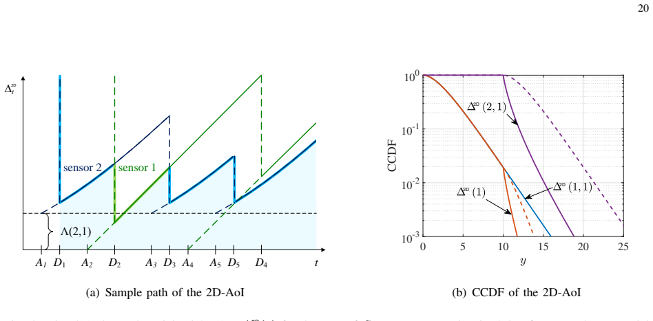
The machinery is Gaussian-process prediction under a product kernel $k(\varsigma,s,\Delta_t) = \sigma^2 g(\Delta_t(\varsigma)) h(\varsigma,s)$, where $g(0)=h(s,s)=1$. The posterior variance of a prediction from a single newest sample is $\Phi_t(\varsigma,s) = \sigma^2(1-(g(\Delta_t)h(\varsigma,s))^2)$. Equating this variance to the variance of a local sample gives the 2D-AoI transformation $\Delta_t^{2D} = g^{-1}(g(\Delta_t) h(\varsigma,s))$, which transfers the spatial correlation into the temporal domain, so that the CCDF of the minimal 2D-AoI factorizes as a product of per-sensor shifted AoI CCDFs (Eq. (7)).
What would settle it
Take a real spatio-temporal dataset, fit an exponential product kernel, and compare the actual mean-squared prediction error of a distant sensor's newest sample with the error of a local sample whose age equals the 2D-AoI from Eq. (16); a systematic mismatch, or a large improvement when all past samples are used, shows the equivalence is an approximation rather than an identity.
Extended reading notes
Core claim
On the paper's own terms: the Age-equivalent Distance (AeD) $\Lambda_t(\varsigma,s)$ is defined through the posterior variance of a Gaussian process, so that using the most recent sample from sensor $\varsigma$ to predict the process at location $s$ yields the same prediction variance as a sample at $s$ that is $\Delta_t^{2D}$ old. The central identity is $\Delta_t^{2D}(\varsigma,s) = g^{-1}(g(\Delta_t(\varsigma)) h(\varsigma,s))$ (Eq. 16), which transfers spatial correlation into the temporal domain. The paper then derives closed-form AeDs for exponential, squared exponential, and rational quadratic product kernels, and plugs them into the CCDF of the minimal 2D-AoI over all sensors, Eq. (7), to evaluate the 2D-AoI of a sensor grid served by independent M/M/1 queues or slotted ALOHA channels, identifying sensor distances $d$ that minimize the expected 2D-AoI under a per-area capacity constraint.
Load-bearing premise
The central identity holds only if the physical process is Gaussian with a known separable product kernel and if the monitor's prediction quality is captured by the posterior variance from the most recent sample alone.
Editorial extensions
If this is right
- The 2D-AoI of a set of sensors with exponential kernels is the AoI of a parallel system with per-sensor offsets $\Lambda(\varsigma,s)=(\ell_t/\ell_s)|x_\varsigma-x_s|$, so existing AoI results for parallel systems transfer immediately.
- The optimal sensor distance $d$ that minimizes the expected 2D-AoI under a per-area capacity budget is finite and grows when the spatial correlation length $\ell_s$ or the per-area service rate $\mu$ increases.
- When a local sensor cannot meet an AoI threshold on its own, a distant sensor can still help, and the required service rate of the local sensor decreases linearly with the distant sensor's rate, discounted by the ratio of the AeD to the threshold (Eq. (12)).
- With squared exponential kernels, samples from distant sensors become relatively more valuable as the local AoI grows, because their age-equivalent offset shrinks with age.
Reading between the lines
- A direct extension of the paper's recipe is that any kernel with a tractable inverse $g^{-1}$ yields an AeD, so the construction generalizes to other covariance families and to mixed spatio-temporal kernels.
- Because the derivation uses only the newest sample, the 2D-AoI is optimistic about prediction quality; the paper's own Fig. 9(c) shows that using all past samples lowers the prediction variance, so a practical monitor should treat the 2D-AoI as an upper bound on the value of the best sample.
- For random sensor positions, the AeD becomes a random variable; treating it as such (as the paper does for overlapping sensors) turns the 2D-AoI into a convolution problem, which connects naturally to stochastic geometry analyses of sensor deployments.
Editorial analysis
A structured set of objections, weighed in public.
Referee Report
Summary. The paper proposes 2D-AoI, an age-of-information metric for spatio-temporal processes monitored by distributed sensors. For Gaussian processes with separable product kernels, it defines the Age-equivalent Distance (AeD) so that a sample from a distant sensor with age Δt(ς) has the same single-sample posterior prediction variance as a local sample of age Δ2D = g^{-1}(g(Δt(ς)) h(ς,s)) (Eq. 16). Closed-form AeDs are derived for exponential, squared-exponential, and rational-quadratic kernels, and CCDFs of the resulting 2D-AoI are computed for independent M/M/1 queues and slotted ALOHA channels. The framework is applied to a star-topology resource allocation problem and to a regular sensor grid to identify sensor densities that minimize mean 2D-AoI; the final section compares the prediction variance obtained from the best sample with that obtained from all samples.
Significance. The paper's core contribution is a clean reduction of spatial correlation to an age-equivalent quantity, which lets the authors transfer AoI results for parallel systems to spatially distributed correlated sensors. The posterior-variance calculation in Eq. (15) and the kernel-specific derivations in Sec. VI are correct, and the exponential-kernel offset Λ = (lt/ls)|x| and the time-dependent offsets for squared-exponential and rational-quadratic kernels are elegant and potentially useful. The paper also provides explicit CCDFs that can be reused with other channel models, and it includes a random-AeD extension in Appendix IX-D. The main caveat, which the paper itself documents in Sec. VII-C, is that the 2D-AoI objective is based on the most recent sample only, whereas the monitor can fuse all available samples; whether the density optima survive under full-sample GP fusion is not established.
major comments (1)
- [Sec. VII-C and Table I; Eq. (4) vs Eq. (13)] The sensor-density optima in Figs. 7 and 8 minimize E[Δ2D] under the single-best-sample selection rule (4), but Eq. (13) and Fig. 9(c) show that using all available samples reduces the posterior variance; for d=40 and ls=128, E[Φ] drops from 0.597 to 0.553 (Table I). The paper does not show that the d that minimizes E[Δ2D] also minimizes the full-sample posterior variance E[Φ_all]. Moreover, even under best-sample selection, Φ = σ2(1 − g(Δ2D)2) (Eq. 17) is a nonlinear function of Δ2D, so the minimizer of E[Δ2D] need not minimize E[Φ]. Since the paper's design claims are about optimizing sensor density for monitoring a spatio-temporal process, the optima in Figs. 7 and 8 could be artifacts of discarding information. The authors should either prove the coincidence of the minimizers for the considered kernels and channels, or explicitly frame the optima as minimizing the single-sample 2D-AoI and add a sensitivity analysis of the optimal d under full-sample GP fusion.
minor comments (5)
- [Abstract and Sec. VI-A] The abstract and Sec. VI-A say that for exponential product kernels 'we find' that spatial distance causes an additive offset; Eq. (22) follows by direct substitution from the definition in Eq. (16). Please phrase this as a consequence of the definition rather than an empirical discovery.
- [Sec. III vs Sec. VII] The symbol S is used both for the set of sensors (Sec. III) and for the number of nearest sensors (Sec. VII and Fig. 6). Use a different symbol for one of these to avoid confusion.
- [Eq. (7)] Eq. (7) should state explicitly that for y < Λ(ς,s) the factor P[Δt(ς) > y − Λ(ς,s)] equals 1; Eq. (19) includes this condition, but Sec. IV does not.
- [Fig. 3(c)] The caption of Fig. 3(c) does not explain the meaning of the '(y,ε)' goal point or the slopes labeled μ1/2 and μ2/2; please clarify the construction in the text.
- [Sec. VII-C] The all-samples simulation in Fig. 9(c) uses a finite horizon T=1000; please justify that this truncation does not affect the comparison, for example by reporting the probability that a sensor's latest sample is older than T for the parameters considered.
Circularity Check
No significant circularity: the kernel-specific AeD formulas are direct consequences of the explicitly defined age-equivalent mapping, not fitted or self-referential predictions.
full rationale
The paper explicitly defines the 2D-AoI in Eq. (16) as Δ2D = g^{-1}(g(Δt)h(ς,s)), deliberately chosen so that the single-sample Gaussian-process prediction variance in Eq. (15) becomes σ²(1 − g(Δ2D)²). The subsequent AeD formulas for the exponential kernel (Eq. 22) and squared-exponential kernel (Eq. 25) are obtained by substituting the stated kernel functions into this definition; they are analytic identities under the stated kernel assumptions, presented transparently as consequences of the definition rather than as empirical discoveries. No parameter is fitted to a target quantity and then renamed a prediction: kernel length scales and queue/channel parameters are assumed inputs, and the M/M/1 AoI CCDF in Eq. (9) is taken from the external reference [12]. The parallel-system minimum structure in Eq. (7) is standard and independently cited ([6], [50]); any self-citations are not load-bearing for the central equivalence. The acknowledged single-sample restriction, along with the Fig. 9(c) observation that all-sample GP fusion lowers prediction variance, is a limitation of the metric's scope, not circular reasoning: the paper consistently evaluates 2D-AoI for the most recent sample and explicitly notes in Sec. V-A that the monitor can still use all available samples in Eq. (13). Thus the derivation chain is self-contained with respect to its stated definitions and assumptions.
Assumptions & free parameters
free parameters (6)
- temporal length scale lt =
lt = 128 (Sec. VII)
- spatial length scale ls =
ls in {64, 128, 256, 512, infinity}
- M/M/1 utilization rho =
rho = 0.53
- number of nearest sensors S =
S = 16 (and 36 in appendix)
- area size A =
A = 300^2
- process variance sigma^2 =
sigma^2 = 1
assumptions (5)
- domain assumption The monitored phenomenon is a Gaussian process with zero mean and known covariance kernel (Sec. V-A).
- domain assumption The correlation kernel is a separable stationary product of a temporal kernel g and a spatial kernel h with g(0)=h(s,s)=1 and g decreasing (Eq. 14).
- domain assumption Sample utility is measured by the posterior variance of a prediction using only the most recent sample from each sensor (Sec. V-A, V-B).
- domain assumption Each sensor is connected to the monitor by an independent channel, so the CCDF of the minimum factors into a product (Eq. 6).
- standard math The M/M/1 and slotted ALOHA AoI CCDFs from prior work are correct (Eqs. 9 and 28).
invented entities (1)
-
2D-AoI and Age-equivalent Distance (AeD)
Cite this review
Pith. "Pith review of 2D-AoI: Age-of-Information of Distributed Sensors for Spatio-Temporal Processes." pith.science (2026). https://pith.science/paper/KS5KPYAK
@misc{pith2026241212789,
  author       = {Pith},
  title        = {Pith review of: 2D-AoI: Age-of-Information of Distributed Sensors for Spatio-Temporal Processes},
  year         = {2026},
  howpublished = {\url{https://pith.science/paper/KS5KPYAK}},
  note         = {Machine review of arXiv:2412.12789}
}
read the original abstract
The freshness of sensor data is critical for all types of cyber-physical systems. An established measure for quantifying data freshness is the Age-of-Information (AoI), which has been the subject of extensive research. Recently, there has been increased interest in multi-sensor systems: redundant sensors producing samples of the same physical process, sensors such as cameras producing overlapping views, or distributed sensors producing correlated samples. When the information from a particular sensor is outdated, fresh samples from other correlated sensors can be helpful. To quantify the utility of distant but correlated samples, we put forth a two-dimensional (2D) model of AoI that takes into account the sensor distance in an age-equivalent representation. Since we define 2D-AoI as equivalent to AoI, it can be readily linked to existing AoI research, especially on parallel systems. We consider physical phenomena modeled as spatio-temporal processes and derive the 2D-AoI for different Gaussian correlation kernels. For a basic exponential product kernel, we find that spatial distance causes an additive offset of the AoI, while for other kernels the effects of spatial distance are more complex and vary with time. Using our methodology, we evaluate the 2D-AoI of different spatial topologies and sensor densities.
Figures


Figures from the paper (7 more)



Forward citations
Cited by 1 Pith paper
-
Spatio-Temporal Information Freshness for Remote Source Monitoring in IoT Systems
For a slotted ALOHA IoT system with distance-dependent sensor reliability, minimizing conditional entropy yields a smaller optimal coverage radius than minimizing age of information.
Reference graph
Works this paper leans on
-
[1]
Minimizing age of information in vehicular networks,
S. Kaul, M. Gruteser, V . Rai, and J. Kenney, “Minimizing age of information in vehicular networks,” in Proc. of IEEE SECON, Jun. 2011, pp. 350–358
work page 2011
-
[2]
Real-time status: How often should one update?
S. Kaul, R. Yates, and M. Gruteser, “Real-time status: How often should one update?” in Proc. of IEEE INFOCOM Mini-Conference, Mar. 2012, pp. 2731–2735
work page 2012
-
[3]
Age of information: An introduction and survey,
R. D. Yates, Y . Sun, D. R. Brown, S. K. Kaul, E. Modiano, and S. Ulukus, “Age of information: An introduction and survey,” IEEE J. Sel. Areas Commun. , vol. 39, no. 5, pp. 1183–1210, May 2021
2021
- [4]
-
[5]
Age-optimal scheduling over hybrid channels,
J. Pan, A. M. Bedewy, Y . Sun, and N. B. Shroff, “Age-optimal scheduling over hybrid channels,” IEEE Trans. Mob. Comput., pp. 1–17, 2022
work page 2022
-
[6]
M. Fidler, J. P. Champati, J. Widmer, and M. Noroozi, “Statistical age-of-information bounds for parallel systems: When do independent channels make a difference?” IEEE J. Sel. Topics Inf. Theory , vol. 4, pp. 591–606, Nov. 2023
work page 2023
-
[7]
Optimizing information freshness in wireless networks under general interference constraints,
R. Talak, S. Karaman, and E. Modiano, “Optimizing information freshness in wireless networks under general interference constraints,” IEEE/ACM Trans. Netw., vol. 28, no. 1, pp. 15–28, Feb. 2020
work page 2020
-
[8]
Status updates over unrelaible multiaccess channels,
S. K. Kaul and R. D. Yates, “Status updates over unrelaible multiaccess channels,” in Proc. of IEEE ISIT , 2017, pp. 331–335
work page 2017
Show all 57 references
-
[9]
Delay violation probabiliy and age of information interplay in the two-user multiple access channel,
N. Pappas and M. Kountouris, “Delay violation probabiliy and age of information interplay in the two-user multiple access channel,” in Proc. of IEEE SPAWC Workshop, Jul. 2019, pp. 1–5
2019
-
[10]
Age of information in random access channels,
X. Chen, K. Gatsis, H. Hassani, and S. S. Bidokhti, “Age of information in random access channels,” IEEE Trans. Inf. Theory, vol. 68, no. 10, pp. 6548–6568, Oct. 2022
2022
-
[11]
Age of information in G/G/1/1 systems: Age expressions, bounds, special cases, and optimization,
A. Soysal and S. Ulukus, “Age of information in G/G/1/1 systems: Age expressions, bounds, special cases, and optimization,” IEEE Trans. Inf. Theory , vol. 67, no. 11, pp. 7477–7489, 2021
2021
-
[12]
A general formula for the stationary distribution of the age of information and its application to single-server queues,
Y . Inoue, H. Masuyama, T. Takine, and T. Tanaka, “A general formula for the stationary distribution of the age of information and its application to single-server queues,” IEEE Trans. Inf. Theory , vol. 65, no. 12, pp. 8305–8324, Dec. 2019
2019
-
[13]
The age of information in multihop networks,
A. M. Bedewy, Y . Sun, and N. B. Shroff, “The age of information in multihop networks,” IEEE/ACM Trans. Netw., vol. 27, no. 3, pp. 1248–1257, 2019
2019
-
[14]
A Palm calculus approach to the distribution of the age of information,
A. Rizk and J.-Y . L. Boudec, “A Palm calculus approach to the distribution of the age of information,” IEEE Trans. Inf. Theory, vol. 69, no. 12, pp. 8097–8110, Dec. 2023
2023
-
[15]
On the distribution of AoI for the GI/GI/1/1 and GI/GI/1/2* systems: Exact expressions and bounds,
J. P. Champati, H. Al-Zubaidy, and J. Gross, “On the distribution of AoI for the GI/GI/1/1 and GI/GI/1/2* systems: Exact expressions and bounds,” in Proc. of IEEE INFOCOM , Apr. 2019, pp. 37–45
2019
-
[16]
Statistical guarantee optimization for AoI in single-hop and two-hop FCFS systems with periodic arrivals,
——, “Statistical guarantee optimization for AoI in single-hop and two-hop FCFS systems with periodic arrivals,” IEEE Trans. Commun., vol. 69, no. 1, pp. 365–381, Jan. 2021
2021
-
[17]
A min-plus model of age-of-information with worst-case and statistical bounds,
M. Noroozi and M. Fidler, “A min-plus model of age-of-information with worst-case and statistical bounds,” in Proc. of IEEE ICC, 2022
2022
-
[18]
Using correlated information to extend device lifetime,
J. Hribar, M. Costa, N. Kaminski, and L. A. DaSilva, “Using correlated information to extend device lifetime,” IEEE Internet of Things Journal , vol. 6, no. 2, pp. 2439–2448, 2018
2018
-
[19]
Age-driven spatially temporally correlative updating in the satellite-integrated Internet of Things via Markov decision process,
Y . Li, Y . Xu, Q. Zhang, and Z. Yang, “Age-driven spatially temporally correlative updating in the satellite-integrated Internet of Things via Markov decision process,” IEEE Internet of Things Journal , vol. 9, no. 15, pp. 13 612–13 625, 2022
2022
-
[20]
Optimal scheduling of multiple spatiotemporally dependent observations for remote estimation using age of information,
V . W. H˚akansson, N. K. D. Venkategowda, S. Werner, and P. K. Varshney, “Optimal scheduling of multiple spatiotemporally dependent observations for remote estimation using age of information,” IEEE Internet of Things Journal , vol. 9, no. 20, pp. 20 308–20 321, Oct. 2022. 31
2022
-
[21]
Status from a random field: How densely should one update?
Z. Jiang and S. Zhou, “Status from a random field: How densely should one update?” in Proc. of IEEE International Symposium on Information Theory (ISIT) , 2019, pp. 1037–1041
2019
-
[22]
Monitoring correlated sources: AoI-based scheduling is nearly optimal,
R. V . Ramakanth, V . Tripathi, and E. Modiano, “Monitoring correlated sources: AoI-based scheduling is nearly optimal,” in Proc. of IEEE INFOCOM , May 2024
2024
-
[23]
Sampling of the Wiener process for remote estimation over a channel with random delay,
Y . Sun, Y . Polyanskiy, and E. Uysal, “Sampling of the Wiener process for remote estimation over a channel with random delay,” IEEE Trans. Inf. Theory , vol. 66, no. 2, pp. 1118–1135, Feb. 2020
2020
-
[24]
Sampling and remote estimation for the Ornstein-Uhlenbeck process through queues: Age of information and beyond,
T. Z. Ornee and Y . Sun, “Sampling and remote estimation for the Ornstein-Uhlenbeck process through queues: Age of information and beyond,” IEEE/ACM Trans. Netw., vol. 29, no. 5, pp. 1962–1975, 2021
1962
-
[25]
Performance characterization using AoI in a single-loop networked control system,
J. P. Champati, M. Mamduhi, K. Johansson, and J. Gross, “Performance characterization using AoI in a single-loop networked control system,” in Proc. of IEEE INFOCOM AoI Workshop , Apr. 2019, pp. 197–203
2019
-
[26]
AoI-penalty minimization for networked control systems with packet loss,
M. Kl ¨ugel, M. H. Mamduhi, S. Hirche, and W. Kellerer, “AoI-penalty minimization for networked control systems with packet loss,” in Proc. of IEEE INFOCOM AoI Workshop , Apr. 2019, pp. 189–196
2019
-
[27]
Age-of-information vs. value-of-information scheduling for cellular networked control systems,
O. Ayan, M. Vilgelm, M. Kl ¨ugel, S. Hirche, and W. Kellerer, “Age-of-information vs. value-of-information scheduling for cellular networked control systems,” in Proc. of ACM/IEEE ICCPS , Apr. 2019
2019
-
[28]
Forever young: Aging control for hybrid networks,
E. Altman, R. El-Azouzi, D. S. Menasche, and Y . Xu, “Forever young: Aging control for hybrid networks,” in Proc. of ACM Mobihoc, Jul. 2019, pp. 91–100
2019
-
[29]
Update or wait: How to keep your data fresh,
Y . Sun, E. Uysal-Biyikoglu, R. D. Yates, C. E. Koksal, and N. B. Shroff, “Update or wait: How to keep your data fresh,” IEEE Trans. Inf. Theory , vol. 63, no. 11, pp. 7492–7508, Nov. 2017
2017
-
[30]
The age of incorrect information: A new performance metric for status updates,
A. Maatouk, S. Kriouile, M. Assaad, and A. Ephremides, “The age of incorrect information: A new performance metric for status updates,” IEEE/ACM Trans. Netw., vol. 28, no. 5, pp. 2215–2228, Oct. 2020
2020
-
[31]
Age and value of information: Non-linear age case,
A. Kosta, N. Pappas, A. Ephremides, and V . Angelakis, “Age and value of information: Non-linear age case,” in Proc. of IEEE International Symposium on Information Theory (ISIT) , 2017, pp. 326–330
2017
-
[32]
Toward community sensing,
A. Krause, E. Horvitz, A. Kansal, and F. Zhao, “Toward community sensing,” in Proc. of ACM/IEEE IPSN , 2008
2008
-
[33]
Real-time status updating: Multiple sources,
R. D. Yates and S. Kaul, “Real-time status updating: Multiple sources,” in Proc. of IEEE ISIT , 2012, pp. 2666–2670
2012
-
[34]
Age-optimal updates of multiple information flows,
Y . Sun, E. Uysal-Biyikoglu, and S. Kompella, “Age-optimal updates of multiple information flows,” in Proc. of IEEE INFOCOM AoI Workshop, 2018
2018
-
[35]
Age of information in multiple sensing,
A. Javani, M. Zorgui, and Z. Wang, “Age of information in multiple sensing,” in Proc. of IEEE Globecom , 2019
2019
-
[36]
Age-of-information with information source diversity in an energy harvesting system,
E. Gindullina, L. Badia, and D. G ¨und¨uz, “Age-of-information with information source diversity in an energy harvesting system,” IEEE Trans. Green Com. and Netw. , vol. 5, no. 3, pp. 1529–1540, Sep. 2021
2021
-
[37]
Analysis of age of information in dual updating systems,
Z. Chen, D. Deng, H. H. Yang, N. Pappas, L. Hu, Y . Jia, M. Wang, and T. Q. S. Quek, “Analysis of age of information in dual updating systems,” IEEE Trans. Wireless Commun. , vol. 22, no. 11, pp. 8003–8019, Nov. 2023
2023
-
[38]
On the age of information in internet of things systems with correlated devices,
B. Zhou and W. Saad, “On the age of information in internet of things systems with correlated devices,” in Proc. of IEEE Globecom, 2020
2020
-
[39]
Joint assignment and scheduling for minimizing age of correlated information,
Q. He, G. D ´an, and V . Fodor, “Joint assignment and scheduling for minimizing age of correlated information,” IEEE/ACM Trans. Netw., vol. 27, no. 5, pp. 1887–1900, 2019
1900
-
[40]
Minimizing the age of information from sensors with common observations,
A. E. Kalør and P. Popovski, “Minimizing the age of information from sensors with common observations,” IEEE Wireless Communications Letters, vol. 8, no. 5, pp. 1390–1393, 2019
2019
-
[41]
Timely monitoring of dynamic sources with observations from multiple wireless sensors,
——, “Timely monitoring of dynamic sources with observations from multiple wireless sensors,” IEEE/ACM Trans. Netw., vol. 31, no. 3, pp. 1263–1276, Jun. 2023
2023
-
[42]
Optimizing age of information with correlated sources,
V . Tripathi and E. Modiano, “Optimizing age of information with correlated sources,” in Proc. of ACM MobiHoc , Oct. 2022. 32
2022
-
[43]
Age-of-information oriented scheduling for multichannel IoT systems with correlated sources,
J. Tong, L. Fu, and Z. Han, “Age-of-information oriented scheduling for multichannel IoT systems with correlated sources,” IEEE Trans. Wireless Commun. , vol. 21, no. 11, pp. 9775–9790, Nov. 2022
2022
-
[44]
Focusing on information context for ITS using a spatial age of information model,
J. Heinovski, J. T. G ´omez, and F. Dressler, “Focusing on information context for ITS using a spatial age of information model,” Computer Communications, vol. 209, pp. 203–216, 2023
2023
-
[45]
Modeling value of information in remote sensing from correlated sources,
A. Zancanaro, G. Cisotto, and L. Badia, “Modeling value of information in remote sensing from correlated sources,” Computer Communications, vol. 203, pp. 289–297, Apr. 2023
2023
-
[46]
Goal-oriented scheduling in sensor networks with application timing awareness,
J. Holm, F. Chiariotti, A. E. Kalør, B. Soret, T. B. Pedersen, and P. Popovski, “Goal-oriented scheduling in sensor networks with application timing awareness,” IEEE Trans. Commun. , vol. 71, no. 8, pp. 4513–4527, Aug. 2023
2023
-
[47]
Semantic-aware remote estimation of multiple Markov sources under constraints,
J. Luo and N. Pappas, “Semantic-aware remote estimation of multiple Markov sources under constraints,” Tech. Rep. arXiv:2403.16855v1, Mar. 2024
2024 arXiv
-
[48]
Cost and correlation in strategic wireless sensing driven by age of information,
L. Crosara and L. Badia, “Cost and correlation in strategic wireless sensing driven by age of information,” in Proc. of European Wireless Conference, Sep. 2022
2022
-
[49]
Analytical evaluation of age of information in networks of correlated sources,
L. Crosara, A. Zancanaro, G. Cisotto, N. Laurenti, and L. Badia, “Analytical evaluation of age of information in networks of correlated sources,” in IEEE Workshop on Metrology for Agriculture and Forestry , Nov. 2022, pp. 323–328
2022
-
[50]
On the age of information of a queuing system with heterogeneous servers,
A. Bhati, S. R. B. Pillai, and R. Vaze, “On the age of information of a queuing system with heterogeneous servers,” in National Conference on Communications, Kanpur, India , 2021
2021
-
[51]
C. E. Rasmussen and K. I. Williams, Gaussian Processes for Machine Learning . MIT Press, 2006
2006
-
[52]
Automatic model construction with gaussian processes,
D. K. Duvenaud, “Automatic model construction with gaussian processes,” Ph.D. dissertation, Univ. of Cambridge, Jun. 2014
2014
-
[53]
Gaussian processes,
R. Turner, “Gaussian processes,” https://www.youtube.com/watch?v=92-98SYOdlY, Nov. 2016. [Online]. Available: https://www.youtube.com/watch?v=92-98SYOdlY
2016
-
[54]
B. R. Haverkort, Performance of Computer Communication Systems: A Model-Based Approach . Wiley, 1998. IX. A PPENDIX A. Background on Gaussian Process Regression The following Gaussian regression model is commonly used for prediction in machine learning applications [51]. For a...
1998
-
[55]
The Gaussian process is completely specified by its mean function m(x) = E[f (x)] and covariance function k(x, x′) = E[(f (x) − m(x))(f (x′) − m(x′))]
Process Definition: We consider a Gaussian process f (x) that takes an input vector x to a function value f. The Gaussian process is completely specified by its mean function m(x) = E[f (x)] and covariance function k(x, x′) = E[(f (x) − m(x))(f (x′) − m(x′))]. The covariance f...
-
[56]
Regression/Prediction: Given a set of m observed values f, the goal is to predict a set of m∗ values f∗ that are not observed. The joint prior distribution of f and f∗ is f f∗ ∼ N µµµf µµµf∗ , Σff Σff ∗ Σf∗f Σf∗f∗ , where Σff ∗ is the m × m∗ cova...
-
[57]
In brief, the kernel models the degree of similarity between data points
Multi-dimensional Kernels: The choice of the process covariance function, i.e., the kernel, is a much-considered question. In brief, the kernel models the degree of similarity between data points. The kernel can be estimated from training data or it can be defined by a model. ...
Reviewed August 11, 2026 · model on record in the stance chip above.
Discussion (0). Continue with ORCID to comment.