REVIEW 2 major objections 5 minor 2 cited by
nDspec is a Python library that models X-ray spectra, variability power, and energy-dependent lags in one operator-based framework, demonstrated on a bright black hole binary with clear diagnosis of where simple models fail.
Reviewed by Pith at T0; open to challenge. T0 means a machine referee read the full paper against a public rubric. the ladder, T0–T4 →
nDspec is a modular Python framework for forward-modelling multi-dimensional X-ray data, demonstrated on spectral-timing fits to a NICER observation of a black hole X-ray binary.
T0 review reviewed 2026-08-03 challenge →
load-bearing objection A solid, honest software-release paper for a genuinely missing modular spectral-timing framework; the demo shows what works and what doesn't, and the linearity caveat is standard and stated, not fatal. the 2 major comments →
nDspec: a new Python library for modelling multi-dimensional datasets in X-ray astronomy
The pith
A machine-rendered reading of the paper's core claim, the machinery that carries it, and where it could break.
The reading
Core claim
nDspec's central claim is that the linear impulse-response formalism, embedded in an operator-based software design, is sufficient to build a general-purpose framework for multi-dimensional X-ray modelling. The time-dependent flux in an energy band is written f(E,t) = s(t) ⊛ g(E,t): a driving variability signal convolved with an energy- and time-dependent impulse response. In the Fourier domain the cross spectrum between any band and a reference band becomes C(E,ν) = P(ν) G(E,ν) G*(E_ref,ν) — all energy dependence of timing products is carried by the transfer function G(E,ν), while the driving power spectrum P(ν) acts as a frequency-dependent weight. The library chains operator classes that
What carries the argument
Two elements carry the argument. First, the linear impulse response (IRF) formalism: the system's response to a delta-function flash is g(E,t), and its Fourier transform G(E,ν) is the transfer function; the convolution theorem turns time-domain convolution into Fourier-domain multiplication, so cross spectra are computed as C(E,ν) = P(ν) G(E,ν) G*(E_ref,ν). Second, the operator framework: each transformation applied to a model — folding through the detector response matrix, Fourier transformation, power/cross-spectrum construction, comparison with data — is a composable class, so a single model, whether defined in the time domain, as a transfer function, or directly as a cross spectrum, can
Load-bearing premise
The cross-spectrum machinery stands on the assumption that source variability is linear: flux in every energy band is a convolution of one driving signal with a fixed impulse response, so the intrinsic coherence is exactly one and higher-order Fourier products vanish. If a source's variability is significantly nonlinear, predicted lags and cross-spectrum amplitudes will be wrong no matter how good the model components are — a limitation the paper itself acknowledges as beyond
What would settle it
Measure the intrinsic coherence of a bright accreting source over a wide range of Fourier frequencies and energies and look for a significant dip below unity where the transfer function is well constrained, or for detectable bispectral power. Because the formalism fixes coherence at unity, such a detection would make any full cross-spectrum fit systematically wrong at those frequencies, independent of the impulse response chosen. A cheaper version: generate a synthetic dataset from a known nonlinear process (multiplicative or squared variability), fit it with the library, and show that no line
If this is right
- The same model component can be fitted simultaneously to a time-averaged spectrum, a power spectrum, and a lag spectrum, pulling constraints from all three observables rather than analysing each dimension in isolation.
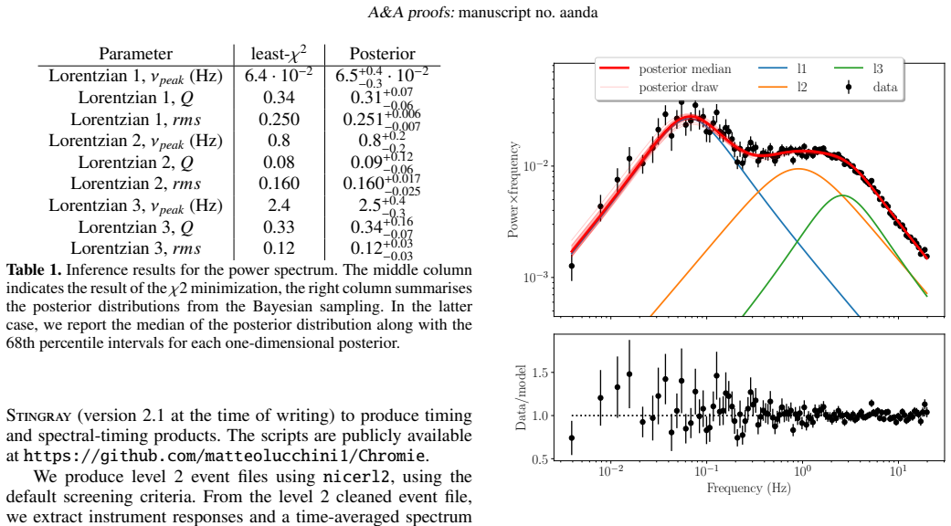
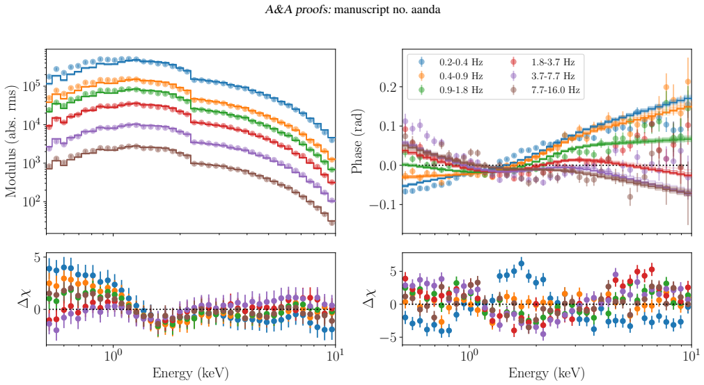
- The demonstration quantifies what current phenomenological models can and cannot do: power spectrum (reduced χ² = 1.05) and energy-dependent lags (reduced χ² = 1.76) fit well, while the full cross spectrum (reduced χ² = 2.99) shows structured residuals at soft energies and near 6 keV, localizing the missing physics to relativistic reverberation.
- Because the Fourier transform can be computed on arbitrary logarithmic grids through a sinc-function decomposition, reverberation models requiring fine time resolution at short delays can be evaluated without uniform oversampling.
- The operator design allows new dimensions — polarimetry, multi-wavelength data, phase-resolved spectra — to be added as new operators and model components, and later releases plan non-Gaussian likelihoods and more advanced sampling methods.
Where Pith is reading between the lines
- The joint pattern of residuals — near 6 keV in both the time-averaged spectrum and the cross-spectrum modulus — suggests the cross-spectrum modulus is a sharper test of reverberation models than phase lags alone; a plausible next step is to make full modulus-plus-phase fits the benchmark for new physical models rather than lag-energy spectra.
- The linearity assumption draws the framework's boundary: any source with intrinsic coherence measurably below unity, or with significant bispectral power, falls outside what the current cross-spectrum class can represent; introducing a coherence parameter or a nonlinear impulse-response treatment would extend the formalism without redesigning the operator chain.
- Because all energy dependence of timing products flows through the transfer function G(E,ν), testing competing geometries (a lamppost corona versus extended Comptonization, for instance) reduces to substituting different impulse responses — a comparison that the current phenomenological components only hint at, but that the operator chain already supports.
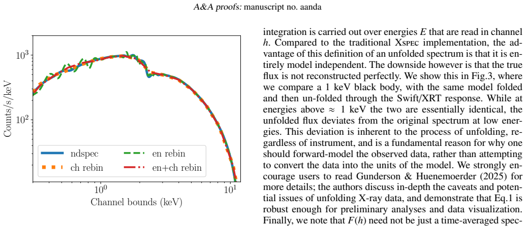
- The paper's repeated warnings about energy-rebinning and unfolding amount to a methodological recommendation: for multi-dimensional products such as rms and lag-energy spectra, forward-folding through the full instrument response is the safe default, and the library is designed around that path.
Editorial analysis
A structured set of objections, weighed in public.
Referee Report
Summary. This paper introduces nDspec, an open-source Python library for forward-modelling multi-dimensional X-ray data. The library currently supports time-averaged spectra, Fourier power spectra, and cross spectra (phase lags, modulus, complex products), using an operator-based architecture: instrument response folding, Fourier transforms (FFT and sinc decomposition), and inference via χ² optimization and emcee MCMC. Unit tests verify response folding against Xspec to 1e-6. The demonstration on a NICER observation of MAXI J1820+070 includes: a 3-Lorentzian fit to the power spectrum (χ²/dof=1.05), a diskbb+powerlaw fit to the time-averaged spectrum (χ²/dof=2.49 with residuals attributed to reflection), and a pivoting-powerlaw + reverberation model fit to energy-dependent phase lags (χ²/dof=1.76). A full modulus+phase cross-spectrum fit is also attempted and fails (χ²/dof=2.99), which the authors interpret as missing relativistic reverberation. Limitations, including the linear IRF assumption and the lack of non-Gaussian likelihoods, are acknowledged.
Significance. The paper addresses a genuine gap: existing X-ray modelling packages are largely 1D or instrument-specific, whereas nDspec provides a modular framework where models, responses, Fourier transforms, and inference are composable. If the software performs as claimed, it will enable joint spectral-timing-polarimetric modelling and is likely to become a useful community tool. Strengths include a reproducibility package (Zenodo), open-source code, and machine-checked agreement with Xspec for response folding. The honest reporting of the failed full cross-spectrum fit is also a strength: it demonstrates that the framework can identify model inadequacy rather than forcing an overparameterized fit. The alpha-release limitations (Gaussian likelihood only, no Xspec wrapper, no polarimetry) are clearly stated and are not obstacles to the underlying design.
major comments (2)
- [Sec. 3.4, phase renormalization] The text contains a direct contradiction. It states 'We begin as previously with least-squares optimization, without enabling the phase re-normalization... The results are shown in Fig.6 and 7; ... χ2/d.o.f.=397.92/226=1.76.' Two paragraphs later: 'we found that enabling the phase renormalization ... improved the quality of all fits without affecting the other parameters, so in the manuscript we only report fits in which it has been enabled.' This makes it impossible to determine whether the reported lag fit (and the corresponding parameters in Table 3) were obtained with or without the six extra phase parameters. Please clarify the exact sequence and state in the figure/table captions which configuration is being reported. This is needed for reproducibility of the central demonstration.
- [Sec. 2.2 / Sec. 3.4, linearity assumption] The cross-spectrum machinery is built on the linear IRF formalism (Eqs. 2–4), which assumes unity intrinsic coherence and zero bispectrum. The paper acknowledges this, but the full cross-spectrum demonstration does not test it. The fit fails with χ2/dof=2.99 and the residuals are interpreted as missing relativistic reverberation. An equally plausible interpretation is that the source variability is nonlinear or intrinsically incoherent, in which case Eq. (4) would be invalid irrespective of the model. I recommend computing the intrinsic coherence of the data (e.g., from the averaged cross spectrum and the two power spectra) or fitting a direct Fourier-domain cross-spectrum model as a control. This would either support the reverberation interpretation or reveal a more fundamental limitation. This is a suggestion to strengthen the interpretation; it does not invalidate the software claim,
minor comments (5)
- [Eq. (4)] The notation S²(ν) should be |S(ν)|²; the power spectrum is |S(ν)|², not S(ν)², since S(ν) is complex. The accompanying text 'S²(ν) is, by definition, the power spectrum' is therefore incorrect.
- [Sec. 2.2, near Eq. (3)] The sentence describing 'the transfer function S(E,ν)' should read G(E,ν); in Eq. (3), S is the transform of the driving signal and G is the transfer function.
- [Table 4] The entry for s_t reports '0+*;* −0.001'; please clarify the notation for a parameter pinned at a limit.
- [Fig. 7 and Fig. 9 captions] The captions describe 'the same model shown in fig.6' and 'fig.8'; this is redundant and can be confusing when figures are viewed separately.
- [Sec. 2.3.1] The text states that only Gaussian uncertainties are supported. It may be worth noting explicitly that χ² fitting of cross-spectrum modulus and phase treats those estimates as Gaussian, which is an approximation for finite integration lengths.
Circularity Check
No significant circularity: nDspec is a forward-modelling software framework whose claims are demonstrated on independent NICER data, with fits and failures reported transparently.
full rationale
No circular step found. nDspec's central claim is that it provides a modular framework for forward-modelling multi-dimensional X-ray data, demonstrated by fitting NICER observations of MAXI J1820+070. These are genuine fits: the power spectrum (chi2/dof=1.05), time-averaged spectrum (2.49), lag spectra (1.76) and full cross spectrum (2.99) are evaluated against the data, and the poor full cross-spectrum fit is reported rather than concealed. The linear impulse response formalism in Sec. 2.2 (Eqs. 2-4) is an explicit modelling assumption, not a derived prediction, and its limitation is openly stated: 'A full treatment of non-linear impulse response functions is beyond the scope of this paper.' The modulus renormalization constants m1-m6 are fitted nuisance parameters, not predictions, and the paper notes their degeneracy with normalization parameters. Self-citations, including Uttley & Malzac (2025) for the sinc transform and phenomenological models, provide algorithms or standard constructs rather than forcing conclusions; the response folding is unit-tested against Xspec to one part in a million, and a reproduction package is provided. Nothing in the paper reduces a claimed result to its own input by construction.
Axiom & Free-Parameter Ledger
free parameters (13)
- gamma_0 =
4.9e-2 (posterior median)
- s_gamma =
-7e-3
- phi_0 =
-1.9
- s_phi =
2.2
- A0 =
6.7 (posterior median, cross-spectrum fit)
- R0 =
115 (posterior median)
- kT0 =
0.272 keV
- s2 =
-2.10 (posterior median)
- st =
0 (pinned to limit)
- tbrk (fixed) =
0.01 s
- s1 (fixed) =
4
- Phi_1..Phi_6 =
approx -0.011, 0.007, 0, 0.011, 0.016, 0.014 rad
- m_1..m_6 =
approx 0.80, 1.38, 0.99, 0.73, 0.84, 1.10
axioms (7)
- domain assumption Flux can be described by a linear impulse response: f(E,t)=s(t) g(E,t) (Eq. 2), so intrinsic coherence is unity and higher-order Fourier products vanish.
- standard math Convolution theorem: the Fourier transform of a convolution is a product (Eq. 3).
- domain assumption Instrument response matrices accurately map incident flux to detector channels and are non-invertible, necessitating forward-folding.
- domain assumption Gaussian (chi-square) likelihood is adequate for the spectral-timing products supported in the alpha release.
- domain assumption Instrumental background is negligible for the bright NICER observation used in the demo.
- domain assumption The sinc-function decomposition (Uttley & Malzac 2025) provides correct Fourier transforms on arbitrary frequency/time grids.
- domain assumption tbabs (Wilms et al. 2000) correctly models interstellar absorption for the demo fits.
Cite this review
Pith. "Pith review of nDspec: a new Python library for modelling multi-dimensional datasets in X-ray astronomy." pith.science (2026). https://pith.science/paper/KXTW6HP7
@misc{pith2026251210615,
  author       = {Pith},
  title        = {Pith review of: nDspec: a new Python library for modelling multi-dimensional datasets in X-ray astronomy},
  year         = {2026},
  howpublished = {\url{https://pith.science/paper/KXTW6HP7}},
  note         = {Machine review of arXiv:2512.10615}
}
read the original abstract
The current fleet of X-ray telescopes produces a wealth of multi-dimensional data, allowing us to study sources in time, photon energy, and polarisation. At the same time, it has become increasingly clear that progress in our physical understanding will only come from studying these sources in multiple dimensions simultaneously. Enabling multi-dimensional studies of X-ray sources requires new theoretical models predicting these datasets, new methods to analyse them, and, crucially, a software framework to combine data, models, and methods efficiently. However, the current ecosystem of software packages developed for X-ray data analysis does not provide the flexibility for advanced modelling of multi-dimensional datasets. In this paper, we introduce nDspec, a new python-based library designed to allow users to seamlessly model one- and multi-dimensional datasets common to X-ray astronomy. Unlike most other libraries, it is designed as a flexible, modular, and extensible framework capable of accommodating multi-dimensional data and able to connect to a range of different inference tools and algorithms. Here we focus on modelling timing and spectral-timing data as a function of both Fourier frequency and energy, in addition to limited support for time-averaged spectra. We discuss design philosophy and current features, and showcase an example use case by characterising a NICER observation of a black hole X-ray binary. We also highlight plans for extensions to other dimensions and new features, such as the inclusion of polarimetry and the improved statistical methods for Bayesian inference.
Figures




Forward citations
Cited by 2 Pith papers
-
Energy-resolved pulse profiles of Vela X-1: cross-calibrating XMM-Newton and NuSTAR to trace spectral features
Pulsed fraction spectra from XMM-Newton and NuSTAR on Vela X-1 agree within 5% after instrumental corrections and reveal emission-line and cyclotron features whose strength varies with orbital absorption.
-
Multi-wavelength outburst activity from EP J174942.2-384834: a very faint X-ray transient discovered by Einstein Probe
EP J174942.2-384834 is classified as a very faint X-ray transient black hole candidate based on its hard X-ray spectra, optical/UV brightening correlated with X-rays, and lack of radio emission.
Reference graph
Works this paper leans on
-
[1]
& Uttley, P
Arévalo, P. & Uttley, P. 2006, MNRAS, 367, 801
2006
-
[2]
Arnaud, K. A. 1996, in Astronomical Society of the Pacific Conference Series, V ol. 101, Astronomical Data Analysis Software and Systems V , ed. G. H. Jacoby & J. Barnes, 17 Astropy Collaboration, Price-Whelan, A. M., Lim, P. L., et al. 2022, ApJ, 935, 167 Astropy Collaboration, Price-Whelan, A. M., Sip˝ocz, B. M., et al. 2018, AJ, 156, 123 Astropy Collab...
1996
-
[3]
2024, Journal of Open Source Software, 9, 7389
Bachetti, M., Huppenkothen, D., Stevens, A., et al. 2024, Journal of Open Source Software, 9, 7389
2024
-
[4]
D., et al
Baldini, L., Bucciantini, N., Lalla, N. D., et al. 2022, SoftwareX, 19, 101194
2022
-
[5]
2022, MNRAS, 515, 2099
Bellavita, C., García, F., Méndez, M., & Karpouzas, K. 2022, MNRAS, 515, 2099
2022
-
[6]
2018, JAX: composable transforma- tions of Python+NumPy programs
Bradbury, J., Frostig, R., Hawkins, P., et al. 2018, JAX: composable transforma- tions of Python+NumPy programs
2018
-
[7]
2021, The Journal of Open Source Software, 6, 3001
Buchner, J. 2021, The Journal of Open Source Software, 6, 3001
2021
-
[8]
2023, Statistics Surveys, 17, 169
Buchner, J. 2023, Statistics Surveys, 17, 169
2023
-
[9]
& Boorman, P
Buchner, J. & Boorman, P. 2023, in Handbook of X-ray and Gamma-ray Astro- physics, 150
2023
-
[10]
2014, A&A, 564, A125
Buchner, J., Georgakakis, A., Nandra, K., et al. 2014, A&A, 564, A125
2014
-
[11]
& Stella, L
Campana, S. & Stella, L. 1995, MNRAS, 272, 585
1995
-
[12]
& Young, A
Chainakun, P. & Young, A. J. 2017, MNRAS, 465, 3965
2017
-
[13]
2020, Proceedings of the National Academy of Science, 117, 30055 De Marco, B., Ponti, G., Petrucci, P
Cranmer, K., Brehmer, J., & Louppe, G. 2020, Proceedings of the National Academy of Science, 117, 30055 De Marco, B., Ponti, G., Petrucci, P. O., et al. 2017, MNRAS, 471, 1475 de Vries, M. N., Wise, M. W., Huppenkothen, D., et al. 2018, MNRAS, 478, 4010 Dupourqué, S., Barret, D., Diez, C. M., Guillot, S., & Quintin, E. 2024, A&A, 690, A317
2020
-
[14]
2025, arXiv e-prints, arXiv:2507.15461
Ewing, M., Ingram, A., Rankin, J., & Muleri, F. 2025, arXiv e-prints, arXiv:2507.15461
Pith/arXiv arXiv 2025
-
[15]
& Hobson, M
Feroz, F. & Hobson, M. P. 2008, MNRAS, 384, 449
2008
-
[16]
P., & Bridges, M
Feroz, F., Hobson, M. P., & Bridges, M. 2009, MNRAS, 398, 1601
2009
-
[17]
P., Cameron, E., & Pettitt, A
Feroz, F., Hobson, M. P., Cameron, E., & Pettitt, A. N. 2019, The Open Journal of Astrophysics, 2, 10
2019
-
[18]
W., Lang, D., & Goodman, J
Foreman-Mackey, D., Hogg, D. W., Lang, D., & Goodman, J. 2013, PASP, 125, 306
2013
-
[19]
2001, in Society of Photo-Optical In- strumentation Engineers (SPIE) Conference Series, V ol
Freeman, P., Doe, S., & Siemiginowska, A. 2001, in Society of Photo-Optical In- strumentation Engineers (SPIE) Conference Series, V ol. 4477, Astronomical Data Analysis, ed. J.-L. Starck & F. D. Murtagh, 76–87
2001
-
[20]
& Calderhead, B
Girolami, M. & Calderhead, B. 2011, Journal of the Royal Statistical Society Series B: Statistical Methodology, 73, 123
2011
-
[21]
Gunderson, S. J. & Huenemoerder, D. P. 2025, AJ, 169, 2
2025
-
[22]
R., Millman, K
Harris, C. R., Millman, K. J., van der Walt, S. J., et al. 2020, Nature, 585, 357
2020
-
[23]
Hunter, J. D. 2007, Computing in Science & Engineering, 9, 90
2007
-
[24]
L., et al
Huppenkothen, D., Bachetti, M., Stevens, A. L., et al. 2019, apj, 881, 39
2019
-
[25]
2022, in Handbook of X-ray and Gamma-ray Astrophysics, ed
Ingram, A. 2022, in Handbook of X-ray and Gamma-ray Astrophysics, ed. C. Bambi & A. Sangangelo, 113
2022
-
[26]
J., Poutanen, J., & Krawczynski, H
Ingram, A., Maccarone, T. J., Poutanen, J., & Krawczynski, H. 2015, ApJ, 807, 53
2015
-
[27]
2016, MNRAS, 461, 1967
Ingram, A., van der Klis, M., Middleton, M., et al. 2016, MNRAS, 461, 1967
2016
-
[28]
Ingram, A. R. & Maccarone, T. J. 2017, MNRAS, 471, 4206
2017
-
[29]
S., Raassen, A
Kaastra, J. S., Raassen, A. J. J., de Plaa, J., & Gu, L. 2025, SPEX X-ray spectral fitting package
2025
-
[30]
2001, MNRAS, 327, 799
Kotov, O., Churazov, E., & Gilfanov, M. 2001, MNRAS, 327, 799
2001
-
[31]
2022, arXiv e-prints, arXiv:2206.09972
Krawczynski, H., Muleri, F., Dov ˇciak, M., et al. 2022, arXiv e-prints, arXiv:2206.09972
Pith/arXiv arXiv 2022
-
[32]
2024, A&A, 686, A259
Lascar, J., Bobin, J., & Acero, F. 2024, A&A, 686, A259
2024
-
[33]
2023, ApJ, 951, 19
Lucchini, M., Mastroserio, G., Wang, J., et al. 2023, ApJ, 951, 19
2023
-
[34]
2018, MNRAS, 475, 4027
Mastroserio, G., Ingram, A., & van der Klis, M. 2018, MNRAS, 475, 4027
2018
-
[35]
2020, MNRAS, 498, 4971
Mastroserio, G., Ingram, A., & van der Klis, M. 2020, MNRAS, 498, 4971
2020
-
[36]
2021, MNRAS, 507, 55 Méndez, M., Peirano, V ., García, F., et al
Mastroserio, G., Ingram, A., Wang, J., et al. 2021, MNRAS, 507, 55 Méndez, M., Peirano, V ., García, F., et al. 2024, MNRAS, 527, 9405
2021
-
[37]
2022, MNRAS, 511, 255
Nathan, E., Ingram, A., Homan, J., et al. 2022, MNRAS, 511, 255
2022
-
[38]
2025, LMFIT: Non-Linear Least- Squares Minimization and Curve-Fitting for Python
Newville, M., Otten, R., Nelson, A., et al. 2025, LMFIT: Non-Linear Least- Squares Minimization and Curve-Fitting for Python
2025
-
[39]
2014, MNRAS, 440, 2882
Rapisarda, S., Ingram, A., & van der Klis, M. 2014, MNRAS, 440, 2882
2014
-
[40]
J., Huppenkothen, D., Lucchini, M., et al
Ricketts, B. J., Huppenkothen, D., Lucchini, M., et al. 2025, MNRAS, 538, 1096
2025
-
[41]
E., Choudhury, D., Salmi, T., et al
Riley, T. E., Choudhury, D., Salmi, T., et al. 2023, Journal of Open Source Soft- ware, 8, 4977
2023
-
[42]
C., et al
Rogantini, D., Costantini, E., Gallo, L. C., et al. 2022, MNRAS, 516, 5171
2022
-
[43]
Shakura, N. I. & Sunyaev, R. A. 1973, A&A, 500, 33
1973
-
[44]
Stevens, A. L. & Uttley, P. 2016, MNRAS, 460, 2796
2016
-
[45]
L., Uttley, P., Altamirano, D., et al
Stevens, A. L., Uttley, P., Altamirano, D., et al. 2018, ApJ, 865, L15
2018
-
[46]
M., Fabian, A
Uttley, P., Cackett, E. M., Fabian, A. C., Kara, E., & Wilkins, D. R. 2014, A&A Rev., 22, 72
2014
-
[47]
& Malzac, J
Uttley, P. & Malzac, J. 2025, MNRAS, 536, 3284
2025
-
[48]
2011, MNRAS, 414, L60 van Paradijs, J
Uttley, P., Wilkinson, T., Cassatella, P., et al. 2011, MNRAS, 414, L60 van Paradijs, J. & Lewin, H. G. 1986, A&A, 157, L10
2011
-
[49]
2010, MNRAS, 402, 307
Vaughan, S. 2010, MNRAS, 402, 307
2010
-
[50]
J., & Castro, D
Vink, J., Patnaude, D. J., & Castro, D. 2022, ApJ, 929, 57
2022
-
[51]
E., et al
Virtanen, P., Gommers, R., Oliphant, T. E., et al. 2020, Nature Methods, 17, 261
2020
-
[52]
2022, ApJ, 930, 18
Wang, J., Kara, E., Lucchini, M., et al. 2022, ApJ, 930, 18
2022
-
[53]
2021, ApJ, 910, L3
Wang, J., Mastroserio, G., Kara, E., et al. 2021, ApJ, 910, L3
2021
-
[54]
R., Cackett, E
Wilkins, D. R., Cackett, E. M., Fabian, A. C., & Reynolds, C. S. 2016, MNRAS, 458, 200
2016
-
[55]
2000, ApJ, 542, 914 Article number, page 13 of 14 A&A proofs:manuscript no
Wilms, J., Allen, A., & McCray, R. 2000, ApJ, 542, 914 Article number, page 13 of 14 A&A proofs:manuscript no. aanda Appendix A: Posterior distributions Here we report the posterior distributions for all the models. Fig..1 shows the corner plot for the fit of the power spectrum. Fig..2 shows the corner plot for the fit of the time-averaged spec- trum. Fig...
arXiv 2000
This paper was first reviewed by deepseek-v4-flash on August 3, 2026.
discussion (0)
Sign in with ORCID, Apple, or X to comment. Anyone can read and Pith papers without signing in.