REVIEW 5 major objections 4 minor 100 references
Spinless glueballs in generalized linear sigma model
T0 review · 5 major / 4 minor · reviewed 2026-08-05 · deepseek-v4-flash
Pith's one-line read A generalized linear sigma model with two pseudoscalar glueball fields reproduces all seven eta masses and finds that η(2225)/X(2370) is almost entirely glue.
desk verdict Strong effort and a new two-glueball construction, but the 'all seven eta masses' claim is an artifact of combining scenarios, and the glue-content conclusion depends on post-hoc filtering. read the letter →
The pith
A machine-rendered reading of the paper's core claim, the machinery that carries it, and where it could break.
The reading
What carries the argument
The central object is the generalized linear $\sigma$ model Lagrangian expanded to leading order in quark/antiquark lines (≤8), containing two chiral nonets $M$ (quark-antiquark) and $M'$ (four-quark), a scalar glueball $h$, and a pseudoscalar glueball $g$. The load-bearing identity is the axial-anomaly ansatz $G=(1-\xi)h^{3}g+\xi h^{3}g'$: integrating out the unphysical $g'$ turns the anomaly into Eq. (15), a linear coupling of $g$ to $\ln(\det M/\det M^{\dagger})$ plus a squared instanton-type term $-c_{3}\xi^{2}[\ln(\det M/\det M^{\dagger})]^{2}$. That squared term supplies the extra U(1)A splitting among the η masses, and the vacuum value $h_0=\langle h\rangle$ controls the glue content of
What would settle it
A decisive observation would be a precise measurement of J/ψ radiative decays into η(2225)/X(2370): a nearly pure pseudoscalar glueball should be produced with a distinctive rate and angular distribution relative to η′(958). If its J/ψ radiative branching ratio matches ordinary quark-antiquark isosinglet expectations, the claim that η(2225) is almost entirely glue is falsified.
Extended reading notes
Core claim
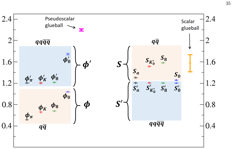
The paper's central claim is that agreement with the seven η masses forces the axial anomaly to be modeled with two pseudoscalar glueballs: a physical one g and an unphysical one g′ integrated out to generate an instanton-type term. With $G=(1-\xi)h^{3}g+\xi h^{3}g'$, integrating out $g'$ gives Eq. (15); at leading order (≤8 quark lines) a 20-parameter Monte Carlo scan then reproduces all seven experimental η masses, favoring η3, η4, η5 = η(1295), η(1760), η(2225). Filtering to the favored high range h0 = 0.65–0.99 GeV, η(2225)/X(2370) is 95% glue, while the scalar glueball content among f0(1370), f0(1500), f0(1710) stays h0-dependent, with the SU(3)-favored h0 ≈ 0.75–0.825 GeV selecting f0(
Load-bearing premise
The whole eta-mass result rests on the assumption that the QCD axial anomaly can be represented by the specific linear combination G=(1−ξ)$h^{3}$ g + ξ $h^{3}$ g′ of two pseudoscalar glueball fields, one unphysical and integrated out; if that combination is not how the anomaly enters the effective Lagrangian, the seven-eta agreement and the glue content of η(2225) do not follow.
Editorial extensions
If this is right
- If the paper is right, η(2225)/X(2370) is the leading experimental candidate for the long-sought pseudoscalar glueball.
- The same Lagrangian gives sizeable glue admixtures to f0(1370), f0(1500), and f0(1710), so pinning down the scalar glueball condensate h0 becomes the decisive next measurement.
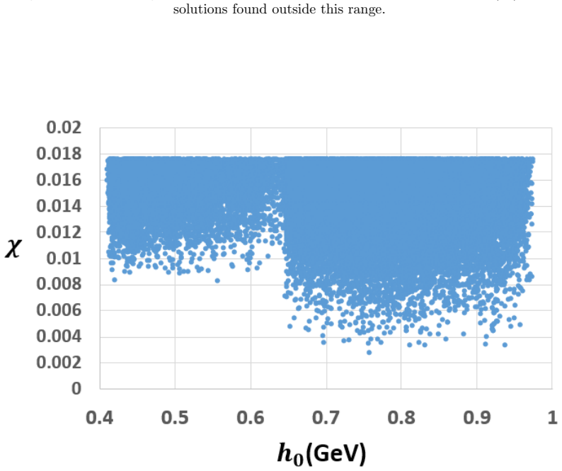
- The simulations split into a low range h0 = 0.40–0.65 GeV and a high range h0 = 0.65–0.99 GeV with contradictory predictions; the decay widths and the SU(3) limit favor the high range, effectively ruling out the low range.
- Because η(2225) and X(2370) differ in mass by only about 3%, either state can serve as the model's fifth pseudoscalar, and the nearly-pure-glue conclusion applies to whatever state occupies that slot.
Reading between the lines
- If the two-glueball anomaly ansatz generalizes, other effective Lagrangians that keep a physical pseudoscalar glueball will also need a second, integrated-out field to preserve the instanton term that drives η–η′ splitting.
- A future lattice QCD value of the scalar glueball condensate at the percent level could decide which f0 is the scalar glueball, since the model's scalar compositions change sharply with h0 even within 0.65–0.99 GeV.
- The near-mass degeneracy of η(2225) and X(2370) means the model cannot assign the glueball label to one uniquely; radiative-decay data could break the degeneracy in a way the mass spectrum alone cannot.
- Because the leading-order truncation yields degenerate bare four-quark nonets, measuring mass splittings among the heavy scalar and pseudoscalar states would test whether subleading terms are needed.
Editorial analysis
A structured set of objections, weighed in public.
Referee Report
Summary. The manuscript develops a generalized linear sigma model with two chiral nonets (quark-antiquark and two-quark-two-antiquark), a scalar glueball h, and a physical pseudoscalar glueball g. To implement the U(1)A anomaly, it additionally introduces an unphysical pseudoscalar glueball g' which is integrated out, yielding an effective instanton-type term. Working at leading order (at most eight quark/antiquark lines) and with a simplified trace anomaly, the author derives 5x5 mass matrices for isosinglet scalars and pseudoscalars, performs a Monte Carlo scan over about 20 parameters, and accepts parameter sets satisfying the chi condition (37) against the experimental eta masses. The paper claims agreement with all seven eta masses, identifies eta(2225) as approximately 95% glue, and analyzes scalar glueball contents and decay widths, ultimately filtering to a high scalar-glueball-condensate range.
Significance. If the claimed agreement were genuine, the framework would be a useful phenomenological tool for glueball-meson mixing. The paper is substantial: it gives explicit mass matrices and three-point couplings, and the numerical scan is extensive. However, the central claim as stated is not supported. The model has only five eta eigenstates; the 'seven eta masses' are reproduced only by stitching together different scenarios. The eta-mass agreement is in-sample because the acceptance condition uses those masses. After filtering, the predicted scalar and kaon masses in Table III deviate by 100-300 MeV from PDG values. The headline glueball assignment depends on discarding the low-h0 region. These issues are load-bearing, so the paper's main conclusions do not follow.
major comments (5)
- [Abstract; Sec. IV.C; Eq. (27); Table I; Fig. 9] The abstract claims the model 'accurately generate[s] all seven eta masses' and is in 'complete agreement with experiment.' Yet the eta mass matrix is 5x5 (Eq. 27), so each parameter set has five eigenstates. The paper itself states 'the model contains five etas' and uses ten assignment scenarios (Table I) to match these to five of the seven PDG states. Fig. 9 shows that eta(1405)/eta(1475) appear only in the low-h0 range (0.40-0.65 GeV) while eta(2225) appears only in the high-h0 range (0.65-0.99 GeV). After filtering to high h0, Table III lists only eta(547), eta'(958), eta(1295), eta(1760), eta(2225). Thus no single parameter set reproduces all seven masses; the apparent complete agreement is an artifact of combining incompatible scenarios.
- [Sec. IV.B-C; Eqs. (35)-(37)] The acceptance condition (37) is built from Eq. (35), which compares the model's eta masses with the experimental eta masses in Eq. (34). Parameter sets are retained only if this chi is below the experimental chi. Consequently, the subsequent 'remarkable agreement' with the eta spectrum is in-sample, not a prediction; the statement in Sec. IV.C that 'this is not a fit' is contradicted by the selection procedure. The model is not independently predicting the eta masses; it is being filtered by them.
- [Table III; Sec. IV.C.1] Table III reports predictions with substantial deviations from PDG values: K0*(700) at 1.116 GeV vs 0.838 GeV, K0*(1430) at 1.576 GeV vs 1.425 GeV, f0(980) at 1.145 GeV vs 0.990 GeV, and f0(1370) around 1.46-1.50 GeV. These are 100-300 MeV off. The text argues that unitarity corrections will lower some of these masses, but those corrections are not computed here. At the level of the Lagrangian masses presented, 'complete agreement with experiment' is not accurate.
- [Sec. VI; Figs. 9, 11; Table IV] The conclusion that eta(2225) is ~95% glue (Table IV) is obtained only after filtering out the low-h0 range (Sec. VI). In the unfiltered scan, Fig. 11 shows that in the low-h0 range eta(1760) carries the largest glue content. The high-h0 filter is justified by decay-width comparisons and other external evidence, but not by a model-internal criterion. The headline assignment therefore depends on choosing one of two contradictory regimes. This is a selection effect, not a robust prediction.
- [Sec. III.A; Eqs. (13)-(15)] The axial anomaly is implemented through the ad hoc combination G=(1-xi)h^3 g + xi h^3 g', with g' an unphysical field having an arbitrary mass and xi a free parameter. Integrating out g' yields the instanton term that drives the eta masses. The paper does not derive this construction from QCD or show it is a controlled approximation to the U(1)A anomaly. Since this term is the main source of the eta masses, the agreement with eta data tests this ansatz, not directly the QCD anomaly. This is a load-bearing assumption that needs independent support.
minor comments (4)
- [Throughout] Typos and spelling errors: 'pseusoscalar', 'tohether', 'antiquak', 'nonlienar sigme model', 'P ARAMETER DETERMINA TION'. A careful proofreading pass is needed.
- [Sec. IV.B] In the sentence 'from the values of u1h2 0, u3h2 0 and u4h2 0', the last combination should presumably be u4 h0 (not u4 h0^2), since u4 was combined with h0 in the previous steps; please clarify notation.
- [Eq. (18)] The displayed expression for fSB appears to have a missing closing parenthesis and ambiguous superscript; please correct the typesetting.
- [Table III] The experimental PDG values in Table III are given with varying precision; for consistency, include the uncertainty of eta(2225) in the table column headers.
Circularity Check
The seven-eta-mass 'agreement' is an in-sample fit: condition (37) selects parameter sets by comparing the five model eta eigenstates to five chosen PDG eta masses, so Table III's eta entries are not predictions; the all-seven claim is also an aggregate over ten scenarios and two h0 ranges that no single parameter set realizes.
-
fitted input called prediction
[Sec. IV B-C, Eqs. (34)-(37), Table I, Fig. 3, Table III]
"To determine each acceptable q, we target experimental values for the eta masses [3]: ... (34). ... χk(p,q) = Σ_i |m theo.[η_i] − m exp.[η_i]| / m exp.[η_i] (35). ... a scenario is considered acceptable if the resulting chi value is less than the corresponding experimental chi value for that scenario. Later: 'Note again that this is not a fit to the experimental data, but rather obtained by imposing the condition (37) which is just a collective constraint on the combination of the eta masses.'"
The acceptance condition (37) is defined by comparing the model's five eta eigenvalues with five of the seven PDG eta masses, for each of the ten assignment scenarios in Table I. Any parameter set retained in S_II is therefore selected precisely because it reproduces a chosen subset of the eta masses. Table III then lists those eta masses as 'predictions', and the abstract reports 'complete agreement' for all seven. This is a fitted input renamed as a prediction: the agreement is in-sample by construction. Additionally, the eta mass matrix is 5×5 (Eq. 27), so no single parameter set has seven eta eigenstates; Fig. 9 shows η(1405)/η(1475) only in the low-h0 range and η(2225) only in the high-h0 range, so the 'all seven' claim is obtained by stitching together incompatible parameter regions
full rationale
The paper's headline claim of reproducing all seven eta masses is the clearest circular step. Equations (34)-(37) make the experimental eta masses the targets of the acceptance filter, and the text explicitly insists this is 'not a fit' even though the goodness function χ_k is a sum of relative mass deviations against those same masses. The ten scenarios in Table I and the h0-dependent results in Fig. 9 further show that the model, having only five eta eigenstates, cannot match all seven PDG states at a single parameter set; the 'complete agreement' is an aggregate over scenarios and h0 ranges. This reduces the central 'all seven eta masses' claim to a fit plus a categorization procedure. The glue-content conclusion for η(2225) is less directly circular: it is an output of the diagonalized mass matrix, but it is obtained only after filtering to the high-h0 range, a filter supported partly by the author's own SU(3)-limit studies [29,30] and partly by decay-width comparisons. Because the decay-width data provide independent filtering support and because the paper does produce genuinely external outputs (kaon masses, f0 masses, decay widths), the circularity is partial rather than total. Score 6 reflects that the central seven-eta prediction reduces by construction, while some independent model content remains.
Assumptions & free parameters
free parameters (10)
- h0 (scalar glueball condensate) =
0.786 GeV average in high range; full acceptable range 0.40-0.99 GeV
- xi (mixing between two pseudoscalar glueballs) =
0.817 +/- 0.100 (Table II)
- gamma1 (log-anomaly mixing parameter) =
0.00655 +/- 0.00188 (Table II)
- c3 (axial anomaly coefficient) =
-4.76e-4 +/- 1.13e-4 (Table II)
- u6 (mass coefficient of physical pseudoscalar glueball) =
4.049 +/- 1.706 (Table II)
- u1, u3, u4 (glueball-nonet couplings) =
Derived from u1 h0^2, u3 h0^2, u4 h0 determined in Appendix A
- u2 (quartic coupling) =
0.388 (Table II)
- alpha1, alpha3, beta1, beta3 (scalar VEVs) =
approx 0.0607, 0.0783, 0.0247, 0.0192 GeV (Table II)
- A1, A3 (quark mass parameters) =
A1 approx 0.000666, A3 approx 0.01955 GeV; A3/A1 constrained to 28.3-30
- gamma_m, lambda1, lambda2, lambda3 (trace anomaly parameters) =
gamma_m=2, lambda1=1/4, lambda2=lambda3=0 (Eq. 21)
assumptions (5)
- domain assumption The two chiral nonets M and M' span the low-energy meson degrees of freedom below about 2 GeV.
- ad hoc to paper Effective terms with at most eight quark and antiquark lines dominate (leading order).
- ad hoc to paper The U(1)A anomaly is exactly modeled by log terms with one physical and one unphysical pseudoscalar glueball, and integrating out the unphysical one yields the instanton term.
- ad hoc to paper The trace anomaly is saturated by the scalar glueball term alone, with lambda1=1/4, lambda2=lambda3=0, gamma_m=2.
- domain assumption Tree-level potential and minimum equations define the vacuum and mass matrices.
invented entities (2)
-
Unphysical pseudoscalar glueball g'
-
Physical pseudoscalar glueball g
independent evidence
Cite this review
Pith. "Pith review of Spinless glueballs in generalized linear sigma model." pith.science (2026). https://pith.science/paper/KYZBOY7M
@misc{pith2026250809474,
  author       = {Pith},
  title        = {Pith review of: Spinless glueballs in generalized linear sigma model},
  year         = {2026},
  howpublished = {\url{https://pith.science/paper/KYZBOY7M}},
  note         = {Machine review of arXiv:2508.09474}
}
read the original abstract
Within the framework of the generalized linear sigma model, a comprehensive analysis of scalar and pseudoscalar glueballs and their mixing with mesons is presented. The Lagrangian of the model contains two chiral nonets, a quark-antiquark type and a two-quark two-antiquark type. The pseudoscalar and scalar glueballs are introduced through their connections with the axial and the trace anomalies of QCD, respectively. It is found that in order to satisfy the axial anomaly and at the same time accurately generate all seven eta masses, it is necessary to include at least two pseudoscalar glueballs, a physical one and an unphysical one that gets integrated out and yields an effective instanton-type term which is needed in generation of the eta masses. At the leading order, which corresponds to keeping effective terms in the Lagrangian that contain no more than eight underlying quarks and antiquarks, the mass spectrum of the model is worked out and shown to be in complete agreement with experiment. The quark and glue contents of the isosinglet scalars below 2 GeV, and of the isosinglet pseudoscalars up to around 2.2 GeV, are analyzed in detail and their correlations with the scalar glueball condensate are examined. Decay widths of isosinglet scalars as well as different self consistencies within this framework are used to probe the glueball condensate and thereby estimate the quark and glue contents of these states. In the pseudoscalar sector, the state that is dominantly made of glue is clearly a state with mass above 2 GeV. In the scalar sector, the identification of glue contents is less certain and in principle the three isosinglets in the 1.5-2.0 GeV can contain substantial glue. These glue contents are determined as functions of the scalar glueball condensate which is the key quantity in this analysis.
Figures


Figures from the paper (19 more)




Reference graph
Works this paper leans on
-
[1]
[69] given in (6)
(27) 9 These mass matrices are subject to the following minimum equations which are obtained from imposing limit (21) on minimum equations (20): ∂V0 ∂fa 0 = 2 √ 2 2u2α3 1 + 2α1β3h0u4 +u 1h2 0α1 + 2α3β1h0u4 −A 1 = 0 ∂V0 ∂fb 0 = 8α 1β1h0u4 + 4u2α3 3 + 2u1h2 0α3 −2A 3 = 0 ∂V0 ∂fc 0 = 2 √ 2h0 (2α1α3u4 +β 1h0u3) = 0 ∂V0 ∂fd 0 = 4α 2 1h0u4 + 2u3h2 0β3 = 0 ∂V0 ∂...
-
[2]
Isodoublet and isotriplet states Although these states have been studied in the framework of the generalized linear sigma model without glueballs in [69], in this section we revisit their case within the present extended framework that has been augmented with glueballs. While glueballs do not directly contribute to these states, as the framework is extend...
-
[3]
Isosinglet states As pointed out before, the properties of the isosinglet states involve both parameterspandqin setS II . Particularly, parameterh 0 (the glueball condensate) plays a key role in this analysis and a range of 0.75-0.825 was favored for this parameter in the analysis of this model in the SU(3) flavor limit in [30]. While we use this SU(3) re...
-
[4]
7 (beyond this range, the model has no acceptable solutions)
Analysis of the glueball condensate over the range ofh0 = 0.40−0.99GeV The histogram forh 0 over its entire range of 0.40−0.99 Gev is given in Fig. 7 (beyond this range, the model has no acceptable solutions). The distribution is consistent with what was found in [29, 30] in the SU(3) limit of this model. We see roughly two ranges,h 0 = 0.40−0.65 GeV (low...
2020
-
[5]
Tr X 2 a − 1 (2u3h2 0)2 det X 2 a −1 = 4u2 4α2 3h2 0 (u3h2 0)2 (A4) which would then allow determination of the combined parametersα 3u4h0 in terms of the combined parametersu 3h2 0 in (A3) and the experimental masses: (α3u4h0)2 = 1 64 (m2 a −m 2 a′)2 − 4 u3h2 0 −(m 2 a +m 2 a′) 2 ! .(A5) Then, the two combined quantities (A3) and (A5), together with the ...
-
[6]
(A6) Next, theπ−π ′ mixing angle is found from the diagonalization ofM 2 π: cos 2θπ = 4 u3h2 0 −m 2 π −m 2 π′ q 64 (α3u4h0)2 + 16 (u3h2 0)2 −8 (u 3h2
-
[7]
37 Next, we compute the combined quantityα 1u4h0 for an input ofA 3/A1 (the ratio of strange to non-strange quark mass)
(m2π +m 2 π′) + (m2π +m 2 π′)2 .(A7) The axial current relates the pion decay constant to the mixing angle: Fπ = 2α1 cosθ π −2β 1 sinθ π (A8) which can then be used to computeα 1 in terms of the known quantities determined above: α1 = 1 2 Fπ cosθ π − β1 α1 sinθ π ,(A9) which in turn determinesβ 1 using the relationship (A6) above. 37 Next, we compute the ...
-
[8]
However, the first three quantities can be in turn expressed in terms of the target quantityα 1u4h0. Usingα 3u4h0 from (A5) andα 1 from (A9), we can expressα 3 in terms of α1u4h0: α3 = (α3u4h0) (α1u4h0) α1 (A11) Using now known quantityu 3h2 0 from (A3),α 1 from (A9), and the fourth minimum equation in (28), we can express β3 in terms ofα 1u4h0: β3 =− 2 (...
Show all 100 references
-
[9]
α1.(A12) Substitutingβ 3 from (A12) into the second equation in (A2), and solving foru 2 we find u2 = 1 8α 2 1 " m2 a +m 2 a′ −m 2 π −m 2 π′ −16 (α1u4h0)2 (u3h2 0) # .(A13) The quantityu 1h2 0 can be expressed in terms ofu 2 in (A13),α 1 in (A9), andu 3h2 0 in (A3). Starting f...
-
[10]
We can also substitute the necessary inputs into (A10) and findA 1 and A3. Furthermore, we can use these combined values to also compute: u4h0 = (u4h0α1) α1 .(A16) In summary, in this appendix we determined parametersα 1, β1, α3, β3, A1, A3, u2 and the combined parameters u1h2...
-
[11]
The interaction Lagrangian and the fields In this appendix we give the notation and formulas for the two-body decay widths of isosinglet scalars into two pseudoscalars. The relevant part of the Lagrangian can be written in the form −L= 1√ 2 X R,A,B γ FR ΠA ΠB FR ΠA ·Π B + 1√ 2...
-
[12]
Decay width formulas The decay widths of isosinglet scalars to two-pseudoscalars are: Γ [FR →Π A ΠB ] = 3 (2−δ AB )γ 2 FR ΠA ΠB q ΠA ΠB 8π m2 FR , Γ [FR →K A KB ] = (2−δ AB )γ 2 FR KA KB q KA KB 8π m2 FR , Γ [FR →η S ηT ] = (1 +δ ST )γ 2 FR ηS ηT qηS ηT 8π m2 FR ,(B15) whereqi...
-
[13]
4α3 1β3 1 γ1 (1 +γ 1) + 6α2 1β2 1 β3α3γ1 (1 +γ 1) +2α1β1β2 3 α2 3 2γ2 1 + 1 +α 3 3β3 3 γ1 # (B48) ∂3V ∂(F 0)2 ∂(η 0)1 ∂(η 0)3 0 =− 4 (2α1β1 +α 3β3)3
Bare couplings The bare coupling constants that are needed in calculation of the physical coupling constats that appear in decay formulas (B16),(B17) and (B18), are directly calculated from the Lagrangian (9) and are given below. * ∂3V ∂(F 0)1 ∂ Π+ 0 1 ∂ Π− 0 1 + 0 = 4 √ 2α1u2...
-
[14]
Fritzsch and M
H. Fritzsch and M. Gell-Mann, eConf C720906V2, 135 (1972). 47
1972
-
[15]
Fritzsch and P
H. Fritzsch and P. Minkowski, Nuovo Cim. A30, 393 (1975)
1975
-
[16]
Navas et al
S. Navas et al. (Particle Data Group), Phys. Rev. D110, 030001 (2024)
2024
-
[17]
See review on ”Spectroscopy of Light Meson Resonances,” in [3]
-
[18]
Vadacchino, in 39th International Symposium on Lattice Field Theory, May 2023
D. Vadacchino, in 39th International Symposium on Lattice Field Theory, May 2023. arXiv: 2305.04869 [hep-lat]
2023 arXiv
- [19]
-
[20]
Llanes-Estrada, Eur
F.J. Llanes-Estrada, Eur. Phys. J. ST230, 1575 (2021)
2021
-
[21]
Pelaez, Phys
J.R. Pelaez, Phys. Rept.658, 1 (2016)
2016
-
[22]
W. Ochs, J. Phys. G40, 043001 (2013)
2013
-
[23]
Klempt and A
E. Klempt and A. Zaitsev, Phys. Rept.454, 1, (2007)
2007
-
[24]
G.S. Bali, K. Schilling, A. Hulsebos, A.C. Irving, C. Michael, and P.W. Stephenson, Phys. Lett. B309, 378 (1993)
1993
-
[25]
Morningstar and M
C.J. Morningstar and M. Peardon, Phys. Rev. D60, 034509 (1999)
1999
-
[26]
Y. Chen, A. Alexandru, S.J. Dong, T. Draper, I. Horvath, F.X. Lee, K.F. Liu, N. Mathur, C. Morningstar and M. Peardon, et al.Phys. Rev. D73, 014516 (2006)
2006
-
[27]
Gregory, A
E. Gregory, A. Irving, B. Lucini, C. McNeile, A. Rago, C. Richards et al., JHEP10, 170 (2012)
2012
-
[28]
F. Chen, X. Jiang, Y. Chen, K.F. Liu, W. Sun and Y.B. Yang, Chin. Phys. C47, 063108 (2023)
2023
-
[29]
Morningstar, PoS LATTICE2024, 004 (2024)
C. Morningstar, PoS LATTICE2024, 004 (2024)
2024
-
[30]
M. A. Shifman, A. I. Vainshtein and V. I. Zakharov, Nucl. Phys. B147, 385 (1979)
1979
-
[31]
Narison, Z
S. Narison, Z. Phys. C26, 209 (1984)
1984
-
[32]
Harnett, R.T
D. Harnett, R.T. Kleiv, K. Moats and T.G. Steele, Nucl. Phys. A850, 110 (2011)
2011
-
[33]
Albaladejo and J
M. Albaladejo and J. A. Oller, Phys. Rev. Lett.101, 252002 (2008)
2008
-
[34]
Nebreda, J
J. Nebreda, J. R. Pelaez and G. Rios, Phys. Rev. D84, 074003 (2011)
2011
-
[35]
Schechter, Phys
J. Schechter, Phys. Rev. D21, 3393 (1979)
1979
-
[36]
Rosenzweig, J
C. Rosenzweig, J. Schechter and C.G. Trahern, Phys. Rev. D21, 3388 (1980)
1980
-
[37]
Rosenzweig, A
C. Rosenzweig, A. Salomone and J. Schechter, Phys. Rev. D24, 2545 (1981)
1981
-
[38]
Janowski, D
S. Janowski, D. Parganlija, F. Giacosa, and D.H. Rischke, Phys. Rev. D84, 054007 (2011)
2011
-
[39]
Eshraim, S
W.I. Eshraim, S. Janowski, F. Giacosa, and D.H. Rischke, Phys. Rev. D87, 054036 (2013)
2013
-
[40]
Fariborz and R
A.H. Fariborz and R. Jora, Phys. Rev. D98, 094032 (2018)
2018
-
[41]
Fariborz and R
A.H. Fariborz and R. Jora, Phys. Lett. B790, 410 (2019)
2019
-
[42]
Fariborz, R
A.H. Fariborz, R. Jora and M. Lyukova, Int. J. Mod. Phys. A34, 1950034 (2019)
2019
-
[43]
Fariborz and M
A.H. Fariborz and M. Lyukova, Nucl. Phys. A1015, 122286 (2021)
2021
-
[44]
Giacosa, S
F. Giacosa, S. Jafarzade and R.D. Pisarski, Phys. Rev. D109, 071502 (2024)
2024
-
[45]
Fariborz, Int
A.H. Fariborz, Int. J. Mod. Phys. A19, 2095-2112 (2004)
-
[46]
A. H. Fariborz, Phys. Rev. D74, 054030 (2006)
2006
-
[47]
Fariborz, A
A.H. Fariborz, A. Azizi and A. Asrar, Phys. Rev. D91, 073013 (2015)
2015
-
[48]
Fariborz, A
A.H. Fariborz, A. Azizi and A. Asrar, Phys. Rev. D92, 113003 (2015)
2015
-
[49]
Meyers and E.S
J. Meyers and E.S. Swanson, Phys. Rev. D87, 036009 (2013)
2013
-
[50]
Sanchis-Alepuz, C.S
H. Sanchis-Alepuz, C.S. Fischer, C. Kellermann, and L. von Smekal, Phys. Rev. D92, 034001 (2015)
2015
-
[51]
Kaptari and B
L. Kaptari and B. Kampfer, Few Body Syst.61, 28 (2020)
2020
-
[52]
Carlson, T.H
C.E. Carlson, T.H. Hansson and C. Peterson, Phys. Rev. D 27, 1556 (1983)
1983
-
[53]
Jaffe, K
R.L. Jaffe, K. Johnson and Z. Ryzak, Annals Phys.168, 344 (1986)
1986
-
[54]
Szczepaniak, E.S
A. Szczepaniak, E.S. Swanson, C.-R. Ji, and S. R. Cotanch, Phys. Rev. Lett.76, 2011 (1996)
2011
-
[55]
Szczepaniak and E.S
A.P. Szczepaniak and E.S. Swanson, Phys. Lett. B577, 61 (2003)
2003
-
[56]
Chanowitz, Phys
M. Chanowitz, Phys. Rev. Lett.95, 172001 (2005)
2005
-
[57]
Dudal, M.S
D. Dudal, M.S. Guimaraes, and S.P. Sorella, Phys. Rev. Lett.106, 062003 (2011)
2011
-
[58]
Windisch, M.Q
A. Windisch, M.Q. Huber and R. Alkofer, Phys. Rev. D87, 065005(2013)
2013
-
[59]
Dudal, M.S
D. Dudal, M.S. Guimaraes, and S.P. Sorella, Phys. Lett. B732, 247?254 (2014)
2014
-
[60]
Fr` ere and J
J.M. Fr` ere and J. Heeck, Phys. Rev. D92, 114035 (2015)
2015
-
[61]
Cheng, C.K
H.Y. Cheng, C.K. Chua and K.F. Liu, Phys. Rev. D92, 094006 (2015)
2015
-
[62]
Huber, C.S
M.Q. Huber, C.S. Fischer and H. Sanchis-Alepuz, Eur. Phys. J. C80, 1077 (2020)
2020
-
[63]
Souza, M.N
E.V. Souza, M.N. Ferreira, A.C. Aguilar, J. Papavassiliou, C.D. Roberts, and S.-S. Xu, Eur. Phys. J. A56, 25 (2020)
2020
-
[64]
Rodas, A
A. Rodas, A. Pilloni, M. Albaladejo, C. Fernandez-Ramrez, V. Mathieu and A.P. Szczepaniakit, Eur. Phys. J. C82, 80 (2022)
2022
-
[65]
Amsler and F.E
C. Amsler and F.E. Close, Phys. Rev.D53, 295 (1996)
1996
-
[66]
Anisovich, V.V
A.V. Anisovich, V.V. Anisovich and A.V. Sarantsev, Phys. Lett.B395, 123 (1997)
1997
-
[67]
Close and A
F.E. Close and A. Kirk, Phys. Lett. B397, 333 (1997)
1997
-
[68]
Narison, Nuclear Physics B509, 312 (1998)
S. Narison, Nuclear Physics B509, 312 (1998)
1998
-
[69]
Close and A
F.E. Close and A. Kirk, Eur. Phys. J. C21, 531 (2001)
2001
-
[70]
Amsler, Phys
C. Amsler, Phys. Lett.B541, 22 (2002)
2002
-
[71]
Close and Q
F.E. Close and Q. Zhao, Phys. Rev. D71, 094022 (2005)
2005
-
[72]
Cheng, C.-K
H.-Y. Cheng, C.-K. Chua and K.-F. Liu, Phys. Rev.D74, 094005 (2006)
2006
-
[73]
Lee and D
W.-J. Lee and D. Weingarten, Phys. Rev.D61, 014015 (2000)
2000
-
[74]
Janowski, F
S. Janowski, F. Giacosa and D.H. Rischke, Phys. Rev.D90, 114005 (2014)
2014
-
[75]
Brnner and A
F. Brnner and A. Rebhan, Phys. Rev. Lett.115, 131601 (2015)
2015
-
[76]
Sarantsevet al., Physics Letters B816, 136227 (2021)
A. Sarantsevet al., Physics Letters B816, 136227 (2021). 48
2021
-
[77]
Rodas et al., Eur
A. Rodas et al., Eur. Phys. J. C82, 80 (2022)
2022
-
[78]
Jaffe, Phys
R.L. Jaffe, Phys. Rev. D15, 267 (1977)
1977
-
[79]
Black, A.H
D. Black, A.H. Fariborz and J. Schechter, Phys. Rev. D61, 074001 (2000)
2000
-
[80]
Black, A.H
D. Black, A.H. Fariborz, S. Moussa, S. Nasri and J. Schechter, Phys. Rev. D64, 014031 (2001)
2001
-
[81]
Fariborz, R
A.H. Fariborz, R. Jora and J. Schechter, Phys. Rev. D72, 034001 (2005)
2005
-
[82]
Fariborz, R
A.H. Fariborz, R. Jora and J. Schechter, Phys. Rev. D79, 074014 (2009)
2009
-
[83]
Fariborz, R
A.H. Fariborz, R. Jora, J. Schechter and M.N. Shahid, Phys. Rev. D84, 113004 (2011)
2011
-
[84]
Fariborz, J
A.H. Fariborz, J. Schechter, S. Zarepour and M. Zebarjad, Phys. Rev. D90, 033009 (2014)
2014
-
[85]
Fariborz, E
A.H. Fariborz, E. Pourjafarabadi, S. Zarepour and S.M. Zebarjad, Phys. Rev. D92, 113002 (2015)
2015
-
[86]
Fariborz, S
A.H. Fariborz, S. Zarepour, E. Pourjafarabadi and S.M. Zebarjad, Eur. Phys. J. C82, 1133 (2022)
2022
-
[87]
Ablikim et al
M. Ablikim et al. [BESIII], Phys. Rev. Lett.106, 072002 (2011)
2011
-
[88]
Fariborz, R
A.H. Fariborz, R. Jora and J. Schechter, Phys. Rev. D77, 094004 (2008)
2008
-
[89]
G.?t Hooft, Phys. Rev. D14, 3432 (1976); Phys. Rev. D18, 2199 (1978)
1976
-
[90]
Albaladejo, J.A
M. Albaladejo, J.A. Oller and L. Roca, Phys. Rev. D82, 094019 (2010)
2010
-
[91]
Aubertet al.[BaBar], Phys
B. Aubertet al.[BaBar], Phys. Rev. D76, 012008 (2007)
2007
-
[92]
Ablikimet al.[BES], Phys
M. Ablikimet al.[BES], Phys. Rev. D72, 092002 (2005)
2005
-
[93]
Anisovich, V.A
V.V. Anisovich, V.A. Nikonov and A.V. Sarantsev, Phys. Atom. Nucl.65, 1545 (2002)
2002
-
[94]
Oller and E
J.A. Oller and E. Oset, Nucl. Phys. A620, 438 (1997). [erratum: Nucl. Phys. A652, 407 (1999).]
1997
-
[95]
Loverreet al., Z
P.F. Loverreet al., Z. Phys. C6, 187 (1980)
1980
-
[96]
Cason, A.E
N.M. Cason, A.E. Baumbaugh, J.M. Bishop, N.N. Biswas, V.P. Kenney, V.A. Polychronakos, R.C. Ruchti, W.D. Shephard and J.M. Watson, Phys. Rev. Lett.41, 271 (1978)
1978
-
[97]
Wetzel, K
W. Wetzel, K. Freudenreich, F.X. Gentit, P. Muhlemann, W. Beusch, A. Birman, D. Websdale, P. Astbury, A. Harckham and M. Letheren, Nucl. Phys. B115, 208 (1976)
1976
-
[98]
Bugg, Eur
D.V. Bugg, Eur. Phys. J. C52, 55 (2007)
2007
-
[99]
Barberis et al, Phys
D. Barberis et al, Phys. Lett. B479, 59 (2000)
2000
-
[100]
Oller, Nucl
J.A. Oller, Nucl. Phys. A727, 353 (2003)
2003
Reviewed August 5, 2026 · model on record in the stance chip above.
Discussion (0). Continue with ORCID to comment.