REVIEW 5 major objections 4 minor 63 references
Efficient Estimation of Regularized Tyler's M-Estimator Using Approximate LOOCV
T0 review · 5 major / 4 minor · reviewed 2026-08-07 · deepseek-v4-flash
Pith's one-line read This paper shows that an approximate leave-one-out loss matches exact LOOCV for selecting the shrinkage coefficient of Regularized Tyler's M-estimator, at a fraction of the cost.
desk verdict ACVL is a sensible and mostly validated approximation for RTME shrinkage selection, but its core stability postulate is unproven and the p>=n evidence is thinner than the text suggests. read the letter →
The pith
A machine-rendered reading of the paper's core claim, the machinery that carries it, and where it could break.
The reading
What carries the argument
The mechanism is the plug-in identity of Equation (20): full-data quadratic-form weights $\widetilde{v}_j = x_j^\top \widehat{S}(\alpha; X_n)^{-1}x_j$ take the place of the leave-one-out weights that would come from refitting RTME on $X_{n\setminus i}$. This converts exact LOOCV's $n$ RTME refits into one full-data fit followed by $n$ cheap weighted-rank-one updates, reducing the cost of evaluating the cross-validated loss at one $\alpha$ from $O(nT(np^2+p^3))$ to $O(T(np^2+p^3))$ up to lower-order terms. The whole construction rests on the estimator's algorithmic stability, stated as Proposition III.1: deleting one sample leaves the scattering estimate and its log-likelihood essentially unchanged.
What would settle it
Take a sample of size $n=100$ with $p=500$ from a multivariate Cauchy distribution, compute the exact LOOCV loss (14) and the approximate loss (22) on the same $\alpha$ grid, and compare their minimizers and their values; if the minimizers differ by more than a small tolerance (e.g., 0.05) or the losses deviate substantially, the paper's central claim that the approximation is near-exact is falsified.
Extended reading notes
Core claim
The central discovery is that the leave-one-out estimate $\widehat{S}(\alpha; X_{n\setminus i})$ can be replaced, for the purpose of cross-validation, by the closed-form plug-in estimate $\widetilde{S}(\alpha; X_{n\setminus i}) = (1-\alpha)\frac{p}{n-1}\sum_{j\ne i} \frac{1}{\widetilde{v}_j}x_jx_j^\top + \alpha T$ with $\widetilde{v}_j = x_j^\top \widehat{S}(\alpha; X_n)^{-1}x_j$, where $\widehat{S}(\alpha; X_n)$ is the full-data RTME. The average loss $\widetilde{L}_{\mathrm{CV}}(X_n, \alpha)$ built from these estimates is claimed to be nearly identical to the exact LOOCV loss $L_{\mathrm{CV}}(X_n, \alpha)$, so that its minimizer $\widehat{\alpha}_{\mathrm{ACVL}}$ is a near-optimal shrinkage coefficient. The approximation is justified by Proposition III.1, which postulates that for large $n$ the log-likelihood of a held-out sample under the full-data estimate and under the leave-one-out estimate differs negligibly. The paper demonstrates this identity empirically over a grid of $\alpha$ values and reports that the resulting choices yield lower LOOCV negative log-likelihood on real datasets than the closed-form baselines.
Load-bearing premise
The approach assumes that removing any single sample from the data changes the fitted scatter matrix so little that weights computed from the full-data fit can stand in for the leave-one-out weights; if this stability fails, the approximate loss will diverge from the exact LOOCV loss.
Editorial extensions
If this is right
- Selecting $\alpha$ by the approximate loss costs a factor of $n$ less than exact LOOCV, making data-dependent shrinkage selection practical for RTME at large $n$.
- Because the method is data-dependent and does not rely on distributional or random-matrix-theory asymptotics, it remains accurate when $p \ge n$ and the data are heavy-tailed, where closed-form estimators tend to over- or under-shrink.
- The approach applies in both the $p > n$ and $n > p$ regimes, and on the Yale B, CIFAR10/100, and USPS datasets it yields the lowest LOOCV negative log-likelihood among the compared estimators.
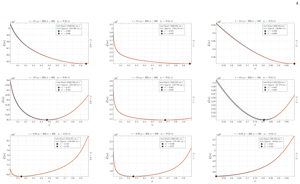
- The approximate loss curves match the exact curves closely across settings, so the same grid search or bisection over $\alpha$ finds essentially the same optimum without invoking the estimator $n$ times.
Reading between the lines
- The stability assumption is most likely to break when $n$ is small relative to $p$ or when the angular distribution is extremely heavy-tailed, since a single sample then carries more directional weight; a systematic study of the exact-versus-approximate loss gap as a function of $p/n$ would test this boundary.
- The same plug-in idea, computing weights once from the full-data estimate and reusing them for leave-one-out, could generalize to other iterative M-estimators and to selection of other hyperparameters, provided a similar stability condition holds.
- The reported 19x to 36x speedups indicate the $O(n)$ saving is real in practice, but the method still evaluates the full-data RTME once per candidate $\alpha$; coupling the approximation with bisection or warm starts should make the total cost nearly independent of grid resolution.
- Because Tyler's estimator and its regularized version operate on normalized directions, the approximate loss inherits scale invariance; this could make the method attractive in applications such as outlier detection and portfolio allocation, where only directions matter.
Editorial analysis
A structured set of objections, weighed in public.
Referee Report
Summary. The paper proposes an approximate leave-one-out cross-validation (LOOCV) procedure, called ACVL, for selecting the shrinkage coefficient α of the Regularized Tyler's M-Estimator (RTME). The exact LOOCV loss (14) requires n RTME fits per candidate α; the paper replaces the leave-one-out fixed-point weights in (17) with full-data weights from (16), yielding the approximate leave-one-out estimate (20) and the ACVL loss (22). The central claims are that (22) closely approximates the exact LOOCV loss (14), that the resulting α is near-optimal, and that the cost is O(n) lower than exact LOOCV. The method is evaluated on synthetic heavy-tailed elliptical data and on several real image datasets, comparing against the shrinkage estimators of Chen-Wiesel-Hero [33] and Zhang-Wiesel [37].
Significance. If the approximation is valid, the ACVL method would provide a practical, data-dependent way to choose the shrinkage coefficient for RTME in high-dimensional settings, where exact LOOCV is prohibitive. The derivation is simple and the reported speedups (roughly 20–35×) are striking. The paper also includes comparisons against existing closed-form and RMT-based methods, with the ACVL method yielding lower NMSE on synthetic data with known ground truth. The main weakness is that the stability assumption underpinning the approximation is stated as a postulate rather than proved, and the empirical evidence lacks repeated trials; these issues currently limit the strength of the claims.
major comments (5)
- [§III-A, Proposition III.1] Proposition III.1 is the load-bearing stability assumption for the entire ACVL derivation, but it is explicitly introduced as a postulate and is not proved. The stated justification — consistency of the loss for fixed p and large n — does not cover the p > n settings used in Section V (e.g., p=200, n=100 and p=500, n=250). Please provide a proof under explicit conditions, or at minimum a quantitative bound on |L(x; \hat S(\bar\alpha; X_n)) − L(x; \hat S(\bar\alpha; X_{n\setminus i}))|, and state the regimes in which the bound holds. As written, the central claim that Eq. (22) approximates Eq. (14) rests on an unverified postulate.
- [§IV, Eq. (20)] Even if the loss is stable under one deletion, the approximation (20) replaces the leave-one-out fixed-point weights \hat v_j in (17) with full-data weights \hat w_j from (16). This is a strictly stronger condition than Proposition III.1: the weights are the mechanism by which RTME downweights influential directions, and in the undersampled regime every sample has high leverage. The synthetic experiments show only one realization per setting, so they do not bound the worst case where a single influential direction shifts the argmin of Eq. (21). Please add a direct comparison of the leave-one-out and full-data weights, or an influence-function analysis, to justify the weight-level replacement.
- [§V, Figures 1–4] The empirical support for the near-identity of the exact and approximate CV losses consists of single generated datasets per configuration; no standard errors, confidence bands, or repeated trials are reported. Since the claim is that the approximation is accurate across settings, please report variability over multiple random seeds (e.g., mean and standard deviation of the loss curves, selected α, and NMSE). Without such replications, the 'almost identical' visual claim in Figures 1 and 2 is not statistically supported.
- [§V, Tables II–V] The real-data evaluation reports the exact LOOCV NLL loss, which is precisely the quantity that ACVL is designed to minimize (through its approximation). It is therefore unsurprising that ACVL achieves the lowest values on this metric, and this does not provide independent evidence of accuracy. Please include a downstream task evaluation (e.g., classification, outlier detection, or a similarly external criterion) or a comparison on data with known ground-truth scatter to support the claim that ACVL is 'consistently more accurate' than other methods.
- [§IV, Eq. (20) and §II-A] The claimed O(n) reduction in running time is not established as written. Computing \tilde S(\bar\alpha; X_{n\setminus i}) separately for each i by summing over j ≠ i in Eq. (20) costs O(n^2 p^2) per \bar\alpha, which is not O(n) faster than exact LOOCV (which costs O(nT(np^2+p^3))). The paper should state that the total weighted sum S_w = \sum_j (1/\hat w_j) x_j x_j^T is computed once and each \tilde S is obtained by subtracting the i-th term, yielding O(np^2+p^3) per \bar\alpha. Without this clarification, the central computational claim is incomplete.
minor comments (4)
- [Table I] The row labels 'Fig. 2' and 'Fig. 3' should refer to 'Fig. 1' and 'Fig. 2'; the current labels are inconsistent with the figure numbering.
- [§V, Figures 1–2] Since the normalized samples x_i = z_i/\|z_i\| do not depend on the scalar u_i, the Cauchy and Gaussian experiments in Figures 1 and 2 are identical in distribution; presenting them as separate heavy-tailed scenarios is redundant and potentially confusing. If the results differ, the authors should explain why, given the cancellation of u_i.
- [§III and §IV] The same symbol bα*_CV is used for the minimizers of the exact loss (13) and the approximate loss (21); please use distinct notation (e.g., bα*_CV and bα*_ACVL) to avoid ambiguity.
- [§V] The convergence criterion for the RFPI algorithm is stated as \|bS − S\|_F < ε, which uses the true scatter S; in practice S is unknown. Please clarify whether this criterion is used only in the synthetic experiments with known S or also in the real-data experiments.
Circularity Check
No significant circularity: ACVL rests on an explicit stability postulate and is validated against external NMSE benchmarks, not on self-citation.
full rationale
The central approximation in Eq. (20) replaces leave-one-out fixed-point weights with full-data weights e_v_j = x_j^T \hat S(alpha; Xn)^{-1} x_j. This is a genuine approximation whose validity the paper attributes to Proposition III.1, an explicitly stated stability postulate, not a theorem derived from the quantity being predicted. In Section III-A the paper writes: "The asymptotic properties of L(Xn; S) encourage us to postulate the following proposition," and the subsequent ACVL loss (22) is compared empirically against exact LOOCV (14) and against the true scatter matrix via NMSE on synthetic data. Those benchmarks are external to the fitted quantity, so the near-identity claim is not forced by construction. The self-citations ([46], [60], [63]) are contextual: [46] is an earlier version of the same proposal, [60] and [63] are general stability references, and none supplies the load-bearing justification for Eq. (20). The main weakness is that Proposition III.1 is unproved and may fail in the p >= n heavy-tail regime used in the experiments; the paper itself acknowledges it is a postulate. That is a correctness and robustness concern, not circularity. Real-data tables score methods by the exact LOOCV NLL objective that ACVL approximates, which mildly favors ACVL, but the synthetic comparisons with the true scatter matrix provide independent content. No equation reduces to its own input, and no fitted parameter is renamed as a prediction.
Assumptions & free parameters
assumptions (5)
- domain assumption Samples x_i are i.i.d. realizations of normalized elliptical vectors with no sample at the origin.
- standard math For alpha > 1 - n/p, the RTME fixed point (10) has a unique solution and the RFPI iteration (11) converges to it.
- ad hoc to paper The regularized Tyler estimator is stable under removal of one sample: L(x; S_hat(alpha; Xn)) is close to L(x; S_hat(alpha; Xn\i)) for large n.
- ad hoc to paper The full-data weights w_hat_i from (16) approximate the leave-one-out weights v_hat_j from (17).
- domain assumption Real image datasets are adequately modeled as heavy-tailed elliptical, so the ACG likelihood is an appropriate scoring rule.
Cite this review
Pith. "Pith review of Efficient Estimation of Regularized Tyler's M-Estimator Using Approximate LOOCV." pith.science (2026). https://pith.science/paper/KZBHXGLO
@misc{pith2026250524781,
  author       = {Pith},
  title        = {Pith review of: Efficient Estimation of Regularized Tyler's M-Estimator Using Approximate LOOCV},
  year         = {2026},
  howpublished = {\url{https://pith.science/paper/KZBHXGLO}},
  note         = {Machine review of arXiv:2505.24781}
}
abstract
We consider the problem of estimating a regularization parameter, or a shrinkage coefficient $\alpha \in (0,1)$ for Regularized Tyler's M-estimator (RTME). In particular, we propose to estimate an optimal shrinkage coefficient by setting $\alpha$ as the solution to a suitably chosen objective function; namely the leave-one-out cross-validated (LOOCV) log-likelihood loss. Since LOOCV is computationally prohibitive even for moderate sample size $n$, we propose a computationally efficient approximation for the LOOCV log-likelihood loss that eliminates the need for invoking the RTME procedure $n$ times for each sample left out during the LOOCV procedure. This approximation yields an $O(n)$ reduction in the running time complexity for the LOOCV procedure, which results in a significant speedup for computing the LOOCV estimate. We demonstrate the efficiency and accuracy of the proposed approach on synthetic high-dimensional data sampled from heavy-tailed elliptical distributions, as well as on real high-dimensional datasets for object recognition, face recognition, and handwritten digit's recognition. Our experiments show that the proposed approach is efficient and consistently more accurate than other methods in the literature for shrinkage coefficient estimation.
Figures


Figures from the paper (2 more)


Reference graph
Works this paper leans on
-
[33]
Robust shrinkage estimation of high-dimensional covariance matrices,
Y . Chen, A. Wiesel, and A. O. Hero, “Robust shrinkage estimation of high-dimensional covariance matrices,” IEEE Trans. on Signal Processing, vol. 59, no. 9, pp. 4097–4107, 2011. 12
work page 2011
-
[37]
Automatic diagonal loading for Tyler’s robust covariance estimator,
T. Zhang and A. Wiesel, “Automatic diagonal loading for Tyler’s robust covariance estimator,” in 2016 IEEE Statistical Signal Processing Workshop, 2016, pp. 1–5
work page 2016
-
[1]
Jolliffe, Principal Component Analysis
I. Jolliffe, Principal Component Analysis . Springer, New York, 2002
work page 2002
-
[2]
The use of multiple measurements in taxonomic problems,
R. A. Fisher, “The use of multiple measurements in taxonomic problems,” Annals of Eugenics , vol. 7, pp. 179–188, 1936
work page 1936
-
[3]
Pareto models for multiclass discriminative linear dimensionality reduction,
K. T. Abou-Moustafa, F. De La Torre, and F. P. Ferrie, “Pareto models for multiclass discriminative linear dimensionality reduction,” Pattern Recognition, vol. 48, no. 5, pp. 1863–1877, 2015
work page 2015
-
[4]
Relations between two sets of variates,
H. Hotelling, “Relations between two sets of variates,”Biometrika, vol. 28, pp. 321–377, 1936
work page 1936
-
[5]
H. Markowitz, “Portfolio selection,” The Journal of Finance , vol. 7, no. 1, pp. 77–91, 1952
work page 1952
-
[6]
P. Rousseeuw and A. Leroy, Eds., Robust Regression and Outlier Detection. Wiley, New York, 1987
work page 1987
Show all 63 references
-
[7]
Multivariate outlier detection based on a robust Mahalanobis distance with shrinkage estimators,
E. Cabana, R. E. Lillo, and H. Laniado, “Multivariate outlier detection based on a robust Mahalanobis distance with shrinkage estimators,” Statistical Papers, vol. 62, no. 4, pp. 1583–1609, Nov 2019
2019
-
[8]
Region covariance: A fast descriptor for detection and classification,
O. Tuzel, F. Porikli, and P. Meer, “Region covariance: A fast descriptor for detection and classification,” in Computer Vision – ECCV 2006 , A. Leonardis, H. Bischof, and A. Pinz, Eds. Springer Berlin Heidelberg, 2006, pp. 589–600
2006
-
[9]
Unified framework to regularized covariance estimation in scaled Gaussian models,
A. Wiesel, “Unified framework to regularized covariance estimation in scaled Gaussian models,” IEEE Trans. on Signal Processing , vol. 60, no. 1, pp. 29–38, 2012
2012
-
[10]
Robust M-Estimators of Multivariate Location and Scatter,
R. A. Maronna, “Robust M-Estimators of Multivariate Location and Scatter,” The Annals of Statistics , vol. 4, no. 1, pp. 51–67, 1976
1976
-
[11]
A Distribution-Free M-Estimator of Multivariate Scatter,
D. E. Tyler, “A Distribution-Free M-Estimator of Multivariate Scatter,” The Annals of Statistics , vol. 15, no. 1, pp. 234–251, 1987
1987
-
[12]
Statistical analysis for the angular central gaussian distribution on the sphere,
——, “Statistical analysis for the angular central gaussian distribution on the sphere,” Biometrika, vol. 74, no. 3, pp. 579–589, 09 1987
1987
-
[13]
Robust and efficient estimation of multivariate scatter and location,
R. A. Maronna and V . J. Yohai, “Robust and efficient estimation of multivariate scatter and location,” Computational Statistics & Data Analysis, vol. 109, pp. 64–75, 2017
2017
-
[14]
Robust estimates of covariance matrices in the large dimensional regime,
R. Couillet, F. Pascal, and J. W. Silverstein, “Robust estimates of covariance matrices in the large dimensional regime,” IEEE Transactions on Information Theory , vol. 60, no. 11, pp. 7269–7278, 2014
2014
-
[15]
Structured robust covariance estimation,
A. Wiesel and T. Zhang, “Structured robust covariance estimation,” Foundations and Trends in Signal Processing , vol. 8, no. 3, pp. 127–216, 2015
2015
-
[16]
Estimation with quadratic loss,
W. James and C. Stein, “Estimation with quadratic loss,” in Proc. of the Fourth Berkeley Symposium on Mathematical Statistics and Probability , vol. 4, no. 1, 1961, pp. 361–379
1961
-
[17]
Estimation of a covariance matrix under stein’s loss,
D. K. Dey and C. Srinivasan, “Estimation of a covariance matrix under stein’s loss,” The Annals of Statistics , vol. 13, no. 4, pp. 1581–1591, 1985
1985
-
[18]
Shrinkage estimators for covariance matrices,
M. J. Daniels and R. E. Kass, “Shrinkage estimators for covariance matrices,” Biometrics, vol. 57, no. 4, pp. 1173–1184, 2001
2001
-
[19]
A well-conditioned estimator for large- dimensional covariance matrices,
O. Ledoit and M. Wolf, “A well-conditioned estimator for large- dimensional covariance matrices,” Journal of Multivariate Analysis , vol. 88, no. 2, pp. 365 – 411, 2004
2004
-
[20]
Empirical Bayes Estimation of the Multivariate Normal Covariance Matrix,
L. R. Haff, “Empirical Bayes Estimation of the Multivariate Normal Covariance Matrix,” The Annals of Statistics , vol. 8, no. 3, pp. 586–597, 1980
1980
-
[21]
First-order methods for sparse covariance selection,
A. d’Aspremont, O. Banerjee, and L. E. Ghaoui, “First-order methods for sparse covariance selection,” SIAM J. Matrix Anal. Appl. , vol. 30, pp. 56–66, 2008
2008
-
[22]
High- dimensional covariance estimation by minimizing L1-penalized log- determinant divergence,
P. Ravikumar, M. J. Wainwright, G. Raskutti, and B. Yu, “High- dimensional covariance estimation by minimizing L1-penalized log- determinant divergence,” Electronic Journal of Statistics , vol. 5, pp. 935–980, 2011
2011
-
[23]
Pourahmadi, High-Dimensional Covariance Estimation , ser
M. Pourahmadi, High-Dimensional Covariance Estimation , ser. Wiley Series in Probability and Statistics. Hoboken, NJ, USA: John Wiley & Sons, 2013
2013
-
[24]
Covariance regularization by thresholding,
P. J. Bickel and E. Levina, “Covariance regularization by thresholding,” The Annals of Statistics , vol. 36, no. 6, pp. 2577–2604, 2008
2008
-
[25]
Spectrum estimation for large dimensional covariance matrices using random matrix theory,
N. E. Karoui, “Spectrum estimation for large dimensional covariance matrices using random matrix theory,” The Annals of Statistics , vol. 36, no. 6, pp. 2757–2790, 2008
2008
-
[26]
Minimax estimation of large covariance matrices under ℓ1-norm,
T. Cai and H. H. Zhou, “Minimax estimation of large covariance matrices under ℓ1-norm,” Statistica Sinica, 2012
2012
-
[27]
Statistical analysis of latent generalized correlation matrix estimation in transelliptical distribution,
F. Han and H. Liu, “Statistical analysis of latent generalized correlation matrix estimation in transelliptical distribution,” Bernoulli, vol. 23, no. 1, pp. 23 – 57, 2017
2017
-
[28]
Huber, Ed., Robust Statistics
P. Huber, Ed., Robust Statistics . Wiley series in Probability and Mathematical Statistics, 1981
1981
-
[29]
F. R. Hampel, E. M. Ronchetti, P. J. Rousseeuw, and W. A. Stahel, Robust Statistics: The Approach Based on Influence Functions , ser. Wiley Series in Probability and Statistics. Hoboken, NJ, USA: John Wiley & Sons, 2011
2011
-
[30]
Distribution theory of spherical distributions and a location- scale parameter generalization,
D. Kelker, “Distribution theory of spherical distributions and a location- scale parameter generalization,” Sankhy¯a: The Indian Journal of Statistics, Series A (1961-2002) , vol. 32, no. 4, pp. 419–430, 1970
1961
-
[31]
On the theory of elliptically contoured distributions,
S. Cambanis, S. Huang, and G. Simons, “On the theory of elliptically contoured distributions,” Journal of Multivariate Analysis , vol. 11, no. 3, pp. 368–385, 1981
1981
-
[32]
Diagonally loaded normalised sample matrix inversion (LNSMI) for outlier-resistant adaptive filtering,
Y . I. Abramovich and N. K. Spencer, “Diagonally loaded normalised sample matrix inversion (LNSMI) for outlier-resistant adaptive filtering,” in 2007 IEEE Int. Conf. on Acoustics, Speech and Signal Processing - ICASSP, vol. 3, 2007, pp. 1105–1108
2007
-
[34]
Generalized robust shrinkage estimator and its application to STAP detection problem,
F. Pascal, Y . Chitour, and Y . Quek, “Generalized robust shrinkage estimator and its application to STAP detection problem,” IEEE Trans. on Signal Processing , vol. 62, no. 21, pp. 5640–5651, 2014
2014
-
[35]
Regularized Tyler’s scatter estimator: Existence, uniqueness, and algorithms,
Y . Sun, P. Babu, and D. P. Palomar, “Regularized Tyler’s scatter estimator: Existence, uniqueness, and algorithms,” IEEE Trans. on Signal Processing, vol. 62, no. 19, pp. 5143–5156, 2014
2014
-
[36]
Regularized M-estimators of scatter matrix,
E. Ollila and D. E. Tyler, “Regularized M-estimators of scatter matrix,” IEEE Trans. on Signal Processing , vol. 62, no. 22, pp. 6059–6070, 2014
2014
-
[38]
Regularized covariance matrix estimation in complex elliptically symmetric distributions using the expected likelihood approach—part 2: The under-sampled case,
O. Besson and Y . I. Abramovich, “Regularized covariance matrix estimation in complex elliptically symmetric distributions using the expected likelihood approach—part 2: The under-sampled case,” IEEE Transactions on Signal Processing, vol. 61, no. 23, pp. 5819–5829, 2013
2013
-
[39]
Optimal shrinkage covariance matrix es- timation under random sampling from elliptical distributions,
E. Ollila and E. Raninen, “Optimal shrinkage covariance matrix es- timation under random sampling from elliptical distributions,” IEEE Transactions on Signal Processing, vol. 67, no. 10, pp. 2707–2719, 2019
2019
-
[40]
Shrinking the eigenvalues of M-estimators of covariance matrix,
E. Ollila, D. P. Palomar, and F. Pascal, “Shrinking the eigenvalues of M-estimators of covariance matrix,” IEEE Transactions on Signal Processing, vol. 69, no. 12, pp. 256–269, 2021
2021
-
[41]
Optimal shrinkage for robust covariance matrix estimators in a small sample size setting,
K. Ashurbekova, A. Usseglio-Carleve, F. Forbes, and S. Achard, “Optimal shrinkage for robust covariance matrix estimators in a small sample size setting,” March 2021, working paper or preprint. [Online]. Available: https://hal.archives-ouvertes.fr/hal-02378034
2021
-
[42]
Large dimensional analysis and optimization of robust shrinkage covariance matrix estimators,
R. Couillet and M. McKay, “Large dimensional analysis and optimization of robust shrinkage covariance matrix estimators,” Journal of Multivariate Analysis, vol. 131, pp. 99–120, 2014
2014
-
[43]
A subspace approach for shrinkage parameter selection in undersampled configuration for regularised Tyler estimators,
Q. Hoarau, A. Breloy, G. Ginolhac, A. Atto, and J. Nicolas, “A subspace approach for shrinkage parameter selection in undersampled configuration for regularised Tyler estimators,” in 2017 IEEE International Conference on Acoustics, Speech and Signal Processing (ICASSP) , 2017,...
2017
-
[44]
Geodesic convexity and regularized scatter estimators,
L. Dümbgen and D. E. Tyler, “Geodesic convexity and regularized scatter estimators,” 2016. [Online]. Available: https://arxiv.org/abs/1607.05455
2016 arXiv
-
[45]
Robust sparse covariance estimation by thresholding Tyler’s M-estimator,
J. Goes, G. Lerman, and B. Nadler, “Robust sparse covariance estimation by thresholding Tyler’s M-estimator,” The Annals of Statistics , vol. 48, no. 1, pp. 86–110, 2020
2020
-
[46]
Shrinkage coefficient estimation for regualrized tyler’s m-estimator. a leave one out approach,
K. Abou-Moustafa, “Shrinkage coefficient estimation for regualrized tyler’s m-estimator. a leave one out approach,” in IEEE Information Theory Workshop (ITW) , 2023, pp. 335–340
2023
-
[47]
Linear shrinkage estimation of covariance matrices using low-complexity cross-validation,
J. Tong, R. Hu, J. Xi, Z. Xiao, Q. Guo, and Y . Yu, “Linear shrinkage estimation of covariance matrices using low-complexity cross-validation,” Signal Processing, vol. 148, pp. 223–233, 2018
2018
-
[48]
Optimal design of the adaptive normalized matched filter detector using regularized Tyler estimators,
A. Kammoun, R. Couillet, F. Pascal, and M.-S. Alouini, “Optimal design of the adaptive normalized matched filter detector using regularized Tyler estimators,” IEEE Transactions on Aerospace and Electronic Systems , vol. 54, pp. 755–769, 2018
2018
-
[49]
Geodesic convexity and covariance estimation,
A. Wiesel, “Geodesic convexity and covariance estimation,” IEEE Transactions on Signal Processing , vol. 60, no. 12, pp. 6182–6189, 2012
2012
-
[50]
Mar ˇcenko–Pastur law for Tyler’s M-estimator,
T. Zhang, X. Cheng, and A. Singer, “Mar ˇcenko–Pastur law for Tyler’s M-estimator,” Journal of Multivariate Analysis , vol. 149, pp. 114–123, 2016
2016
-
[51]
Some hypothesis tests for the covariance matrix when the dimension is large compared to the sample size,
O. Ledoit and M. Wolf, “Some hypothesis tests for the covariance matrix when the dimension is large compared to the sample size,” The Annals of Statistics, vol. 30, no. 4, pp. 1081 – 1102, 2002
2002
-
[52]
Covariance matrix estimation and classification with limited training data,
J. Hoffbeck and D. Landgrebe, “Covariance matrix estimation and classification with limited training data,” IEEE Trans. on Pattern Analysis and Machine Intelligence , vol. 18, no. 7, pp. 763–767, July 1996
1996
-
[53]
The incredible shrinking covariance estimator,
J. Theiler, “The incredible shrinking covariance estimator,” in Automatic Target Recognition XXII, F. A. Sadjadi and A. Mahalanobis, Eds., vol. 8391, International Society for Optics and Photonics. SPIE, 2012, p. 83910P
2012
-
[54]
Maximum likelihood estimation for the wrapped Cauchy distribution,
J. T. Kent and D. E. Tyler, “Maximum likelihood estimation for the wrapped Cauchy distribution,” Journal of Applied Statistics , vol. 15, no. 2, pp. 247–254, 1988
1988
-
[55]
G. H. Golub and C. F. Van Loan, Matrix Computations, 3rd ed. The Johns Hopkins University Press, 1996
1996
-
[56]
Learning in pattern recognition,
T. M. Cover, “Learning in pattern recognition,” in Methodologies of Pattern Recognition, S. Watanabe, Ed. Academic Press, 1969, pp. 111–132
1969
-
[57]
Amari and H
S.-I. Amari and H. Nagaoka, Methods of Information Geometry , ser. AMS Translations of Mathematical Monographs, V ol. 191. Oxford University Press, 2000
2000
-
[58]
Devroye, L
L. Devroye, L. Györfi, and G. Lugosi, A Probabilistic Theory of Pattern Recognition. Springer, 1996
1996
-
[59]
Algorithmic stability and sanity-check bounds for leave-one-out cross-validation,
M. Kearns and D. Ron, “Algorithmic stability and sanity-check bounds for leave-one-out cross-validation,” Neural Computation, vol. 11, no. 6, pp. 1427–1453, Aug 1999
1999
-
[60]
An exponential tail bound for lq stable learning rules,
K. Abou-Moustafa and C. Szepesvári, “An exponential tail bound for lq stable learning rules,” in Proc. of the 30th Int. Conf. on Algorithmic Learning Theory, ser. Proc. of Machine Learning Research, vol. 98, 2019, pp. 31–63
2019
-
[61]
From few to many: Illumination cone models for face recognition under variable lighting and pose,
A. Georghiades, P. Belhumeur, and D. Kriegman, “From few to many: Illumination cone models for face recognition under variable lighting and pose,” IEEE Trans. PAMI, vol. 23, no. 6, pp. 643–660, 2001
2001
-
[62]
UCI Repository of Machine Learning Databases,
D. Newman, S. Hettich, C. Blake, and C. Merz, “UCI Repository of Machine Learning Databases,” 1998, www.ics.uci.edu/∼mlearn/MLRepository.html
1998
-
[63]
An a Priori Exponential Tail Bound for K–Folds Cross–Validation,
K. Abou-Moustafa and C. Szepesvári, “An a Priori Exponential Tail Bound for K–Folds Cross–Validation,” ArXiv e-prints, June 2017
2017
Reviewed August 7, 2026 · model on record in the stance chip above.
Discussion (0). Sign in to comment.