REVIEW 3 major objections 4 minor 33 references
Noise Flow: Noise Modeling with Conditional Normalizing Flows
T0 review · 3 major / 4 minor · reviewed 2026-08-14 · deepseek-v4-flash
Pith's one-line read Noise Flow models real camera noise with 52% higher likelihood than the standard noise level function.
desk verdict Noise Flow is a compact conditional normalizing flow for raw sensor noise with sound bijections, but the headline NLL and PSNR margins rest on an unstated test-split condition. read the letter →
The pith
A machine-rendered reading of the paper's core claim, the machinery that carries it, and where it could break.
The reading
What carries the argument
The central object is the Noise Flow architecture, a bijective normalizing flow built from three ingredients: a signal-dependent layer $f(x) = s \odot x$ with $s = (\beta_1 I + \beta_2)^{1/2}$, a gain layer that scales by $\gamma(\mathrm{ISO}, m) = \psi_m \, u(\mathrm{ISO})\ \mathrm{ISO}$, and repeated affine-coupling plus $1\times 1$ convolutional steps taken from Glow. The whole map is invertible, so one network serves both as a density model (via the change-of-variables formula) and as a noise sampler (by running the inverse map on a Gaussian draw). This is what lets the paper turn a likelihood improvement directly into better synthetic noise for training a denoiser.
What would settle it
Train Noise Flow on noise patches from some SIDD scenes and evaluate on patches from other SIDD scenes—or from a different smartphone sensor—at the same ISO levels; if the 0.42 nats/pixel margin over the camera NLF collapses, the likelihood claim is driven by train/test patch overlap rather than by true generalization.
Extended reading notes
Core claim
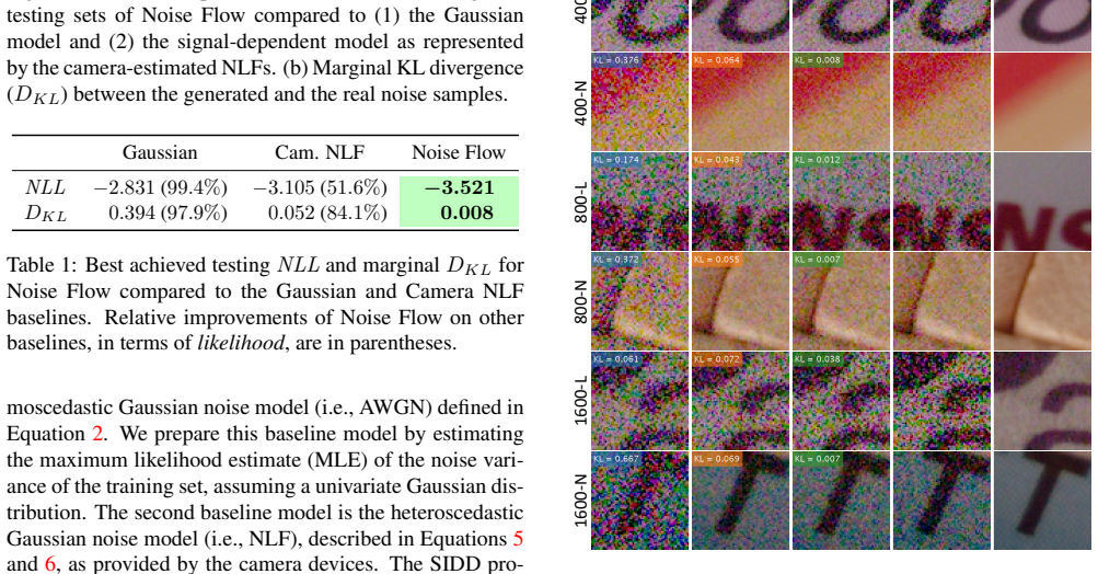
The central claim is that a conditional normalizing flow can serve as a substantially more accurate density model for real sensor noise than the parametric heteroscedastic Gaussian model that is standard in the literature. The flow is explicitly conditioned on intensity through a signal-dependent layer, on ISO through a gain layer, and on camera identity through camera-specific gain weights, and it strictly generalizes the noise level function. The evidence is the NLL comparison in Table 1 and the denoising experiment in Table 3, where synthetic noise from the flow outperforms both hand-crafted parametric noise and real paired data for training a denoiser.
Load-bearing premise
The reported margins rest on the assumption that the 500,000 noise patches are independent representative samples of each camera-ISO-intensity combination, with no clipped or saturated values and no overlap between training and test patches.
Editorial extensions
If this is right
- Noise Flow reproduces and extends the classic NLF: its learned $\beta_1$, $\beta_2$, and $\gamma$ parameters converge to physically sensible values consistent with the signal-dependent model and ISO gain.
- Because the model is compact and camera-specific parameters are isolated in the gain layer, adapting to a new camera requires fine-tuning only those few parameters.
- A denoiser trained purely on Noise Flow-synthesized noise (48.52 dB) outperforms one trained on real noisy/clean pairs from SIDD (47.08 dB), indicating that a good generative noise model can substitute for scarce paired data.
- The flow's invertibility means the same network serves both as a sampler for synthetic noise and as a likelihood model, so progress in likelihood directly translates to progress in synthesis quality.
Reading between the lines
- The current model operates on raw-RGB patches; extending it to sRGB or to full-image spatial correlations across patches would require additional structure, since the coupling layers see only local patches.
- The camera-specific gain weights only adjust a scalar per camera; a camera whose noise behavior differs nonlinearly from the SIDD devices (e.g., a different readout path or on-sensor processing) may need more than fine-tuning that scalar.
- The likelihood gains are measured on SIDD; an immediate test is whether the 0.42 nats/pixel margin persists on another sensor dataset where NLFs might be less well calibrated.
Signed reviews
Editorial analysis
A structured set of objections, weighed in public.
Referee Report
Summary. The paper introduces Noise Flow, a conditional normalizing flow model for image noise that combines Glow-style affine coupling and 1x1 convolutional layers with two new bijective layers: a signal-dependent layer scaling noise by sqrt(beta1*I + beta2) and a gain layer scaling by an ISO- and camera-dependent factor. The model is trained by maximum likelihood on raw-RGB noise patches from the SIDD dataset and is claimed to achieve a test negative log-likelihood of -3.521 nats/pixel, a 0.42 nats/pixel (51.6% likelihood) improvement over the camera-calibrated noise level function, with fewer than 2500 parameters. The paper also applies the model to synthesize training noise for a DnCNN denoiser, reporting 48.52 dB PSNR on SIDD-Validation, above both Gaussian and camera-NLF synthetic baselines and above training on real noisy/clean pairs. The central claims are the density-estimation improvement and the denoising application using synthetic noise.
Significance. If the reported results hold, the paper makes a useful contribution: it demonstrates a principled way to embed well-established parametric noise structures (signal-dependence and gain) into a normalizing flow, yielding a compact and expressive noise model that can be used both for density evaluation and noise synthesis. The authors provide code and pretrained models, and the ablation study (Table 2) gives insight into the contribution of each layer. The key strength is the architectural idea: conditional bijections that exactly generalize the heteroscedastic Gaussian model while allowing arbitrary residual correlations. The main weakness is in the evaluation protocol: the paper does not establish that the test split and the denoising validation are truly out-of-sample with respect to sensor captures and SIDD-Validation images, which is load-bearing for the quantitative claims.
major comments (3)
- [4.1, Table 1] The test NLL evaluation uses a 70/30 split of approximately 500,000 patches, but the paper does not state that the split is by distinct sensor captures or scenes. Since SIDD consists of repeated captures of a small number of scenes, a random patch split very likely places training and test patches from the same raw noisy images. The affine coupling and 1x1 convolutional layers can represent spatially correlated, capture-specific noise (e.g., fixed-pattern noise), so the reported test NLL of -3.521 nats/pixel may reflect in-sample memorization of capture-specific structure rather than generalization to new noise samples. Please specify the exact split procedure; if it is not capture-disjoint, re-run the evaluation with a capture-disjoint split and report the resulting NLL and D_KL.
- [5, Table 3] Noise Flow is described as trained on 'the SIDD' without an explicit statement that the SIDD-Validation images used to evaluate DnCNN-NF were excluded from the Noise Flow training set. If patches from SIDD-Validation were included, the 48.52 dB PSNR is an in-sample result and does not constitute an independent test of synthetic-noise training. Please state the exact subset of SIDD used for Noise Flow training and confirm that it is disjoint from the SIDD-Validation set; if it is not disjoint, retrain Noise Flow on a training-only subset and re-evaluate the denoisers.
- [3.1 and 4.1 (data preparation)] The paper does not describe how clipped or saturated raw pixel values are handled when constructing the noise layers. Clipping is a non-invertible, capture-specific nonlinearity that cannot be represented by the bijective flow layers as defined in Section 3.1. If clipped pixels are present in the training or test patches, the NLL comparison against the Gaussian and NLF baselines may be systematically biased in an uncontrolled way. Please report the fraction of clipped pixels in the train and test sets and either exclude such pixels or explicitly model the clipping process.
minor comments (4)
- [Figure 4(a)] Figure 4(a) is labeled 'NLL (per dimension)' but the vertical axis is positive and decreasing loss corresponds to lower curves, which is consistent with plotting -NLL (i.e., log-likelihood). Please correct the label or plot the actual NLL values, and ensure consistency with Table 1, where NLL values are negative.
- [Section 4.2, Figure 4(b)] The marginal D_KL metric is computed from histograms of pixel values; this ignores all spatial correlations and is sensitive to bin width. Reporting the binning scheme and noting this limitation would help readers interpret the comparison.
- [Throughout] No error bars, confidence intervals, or repeated-seed results are reported for the NLL or PSNR comparisons. Since the test-split methodology is questioned above, reporting variance across multiple random splits or training runs would strengthen the quantitative conclusions.
- [Table 1] The 'improvement in likelihood' percentages are computed by comparing exp(-NLL) values; the text should clarify that this is a likelihood ratio relative to the baseline, not a probability.
Circularity Check
No circularity found: the reported NLL and PSNR gains are empirical maximum-likelihood and hold-out evaluations, not outputs that reduce to the model's own inputs by construction.
full rationale
No circularity was found in the claimed derivation chain. Noise Flow is trained by maximizing the log-likelihood in Equation (8) on SIDD training patches, and the central results in Table 1 (test NLL of -3.521 nats/pixel versus -3.105 for camera NLF) and Table 3 (48.52 dB PSNR for DnCNN-NF) are empirical evaluations on held-out patches and validation images, respectively. The signal-dependent and gain layers in Equations (12) and (14) are parametric components of the model; they are not quantities derived from the same baselines they are compared against. The statement in the introduction that Noise Flow is a strict generalization of the camera NLF is a description of the model family that follows from Equation (12) and the isotropic Normal base measure, but it does not by itself guarantee the reported numerical improvement, which must come from the learned parameters. The learned signal-dependent and gain parameters shown in Figures 6 and 7 are reported after training as consistent with physical expectations; this is post-hoc interpretation, not a prediction, so it does not create a fitted-input-called-prediction issue. The self-citations to the SIDD dataset [1] and to Glow [17] are data and architecture sources, not unverified load-bearing support. The only substantive concerns are experimental rather than circular: the paper does not explicitly state whether the 70/30 patch split is disjoint at the sensor-capture level, nor whether Noise Flow's training distribution excludes the SIDD-Validation images used in the denoising evaluation. These are data-randomization and leakage validity questions, not cases where an equation or fitted parameter is equivalent to the claimed result by construction. Under the rule that circularity requires a specific reduction, the appropriate score is 0.
Assumptions & free parameters
free parameters (5)
- Signal-dependent scale parameters beta1, beta2 =
Learned, not reported numerically
- ISO gain parameters vISO (u=exp(vISO)) =
Learned, not reported numerically
- Camera-specific gain scales psi_m =
Learned, not reported numerically
- Affine coupling and 1x1 convolution weights =
All weights, total fewer than 2500
- Number of flow steps K =
4
assumptions (6)
- standard math The change-of-variables formula (Equation 7) gives the exact likelihood for a composition of differentiable bijections.
- domain assumption The Glow blocks (affine coupling and invertible 1x1 convolution) are bijective with tractable log-determinants.
- domain assumption Noise is additive: observed image equals clean image plus noise layer, with n = noisy minus clean.
- domain assumption Raw-RGB noise is continuous and well modeled by a smooth normalizing flow; clipped or saturated pixels do not require a separate treatment.
- domain assumption The latent clean image used in the signal-dependent layer can be recovered by dividing the SIDD clean image by the learned gain, I = I_gamma / gamma.
- domain assumption SIDD noisy/clean pairs provide ground-truth noise layers.
Cite this review
Pith. "Pith review of Noise Flow: Noise Modeling with Conditional Normalizing Flows." pith.science (2026). https://pith.science/paper/L72HWC7W
@misc{pith2026190808453,
  author       = {Pith},
  title        = {Pith review of: Noise Flow: Noise Modeling with Conditional Normalizing Flows},
  year         = {2026},
  howpublished = {\url{https://pith.science/paper/L72HWC7W}},
  note         = {Machine review of arXiv:1908.08453}
}
read the original abstract
Modeling and synthesizing image noise is an important aspect in many computer vision applications. The long-standing additive white Gaussian and heteroscedastic (signal-dependent) noise models widely used in the literature provide only a coarse approximation of real sensor noise. This paper introduces Noise Flow, a powerful and accurate noise model based on recent normalizing flow architectures. Noise Flow combines well-established basic parametric noise models (e.g., signal-dependent noise) with the flexibility and expressiveness of normalizing flow networks. The result is a single, comprehensive, compact noise model containing fewer than 2500 parameters yet able to represent multiple cameras and gain factors. Noise Flow dramatically outperforms existing noise models, with 0.42 nats/pixel improvement over the camera-calibrated noise level functions, which translates to 52% improvement in the likelihood of sampled noise. Noise Flow represents the first serious attempt to go beyond simple parametric models to one that leverages the power of deep learning and data-driven noise distributions.
Figures


Figures from the paper (5 more)



Reference graph
Works this paper leans on
-
[1]
A High-Quality Denoising Dataset for Smartphone Cameras
Abdelrahman Abdelhamed, Stephen Lin, and Michael S Brown. A High-Quality Denoising Dataset for Smartphone Cameras. In CVPR, 2018. 1, 2, 4, 5, 8
work page 2018
-
[2]
Burst Image Deblur- ring Using Permutation Invariant Convolutional Neural Net- works
Miika Aittala and Fr ´edo Durand. Burst Image Deblur- ring Using Permutation Invariant Convolutional Neural Net- works. In ECCV, 2018. 8
work page 2018
-
[3]
Image Blind Denoising with Generative Adversarial Network Based Noise Modeling
Jingwen Chen, Jiawei Chen, Hongyang Chao, and Ming Yang. Image Blind Denoising with Generative Adversarial Network Based Noise Modeling. In CVPR, 2018. 2
work page 2018
-
[4]
Dirty Pixels: Optimizing Im- age Classification Architectures for Raw Sensor Data
Steven Diamond, Vincent Sitzmann, Stephen Boyd, Gordon Wetzstein, and Felix Heide. Dirty Pixels: Optimizing Im- age Classification Architectures for Raw Sensor Data. arXiv preprint arXiv:1701.06487, 2017. 8
arXiv 2017
-
[5]
NICE: Non-linear Independent Components Estimation
Laurent Dinh, David Krueger, and Yoshua Bengio. NICE: Non-linear Independent Components Estimation. In ICLR Workshop, 2015. 2, 3
work page 2015
-
[6]
Density Estimation using Real NVP
Laurent Dinh, Jascha Sohl-Dickstein, and Samy Bengio. Density Estimation using Real NVP. In ICLR, 2017. 3
work page 2017
-
[7]
Clipped Noisy Images: Heteroskedas- tic Modeling and Practical Denoising
Alessandro Foi. Clipped Noisy Images: Heteroskedas- tic Modeling and Practical Denoising. Signal Processing, 89(12):2609–2629, 2009. 1, 2
work page 2009
-
[8]
Practical Poissonian-Gaussian Noise Modeling and Fitting for Single-Image Raw-Data
Alessandro Foi, Mejdi Trimeche, Vladimir Katkovnik, and Karen Egiazarian. Practical Poissonian-Gaussian Noise Modeling and Fitting for Single-Image Raw-Data. TIP, 17(10):1737–1754, 2015. 1, 2
work page 2015
Show all 33 references
-
[9]
Gow, David Renshaw, Keith Findlater, Lindsay Grant, Stuart J
Ryan D. Gow, David Renshaw, Keith Findlater, Lindsay Grant, Stuart J. McLeod, John Hart, and Robert L. Nicol. A Comprehensive Tool for Modeling CMOS Image-Sensor- Noise Performance. IEEE Transactions on Electron Devices, 54(6):1321–1329, 2007. 4
2007
-
[10]
Noise-Optimal Capture for High Dynamic Range Photogra- phy
Samuel W Hasinoff, Fr ´edo Durand, and William T Freeman. Noise-Optimal Capture for High Dynamic Range Photogra- phy. In CVPR, 2010. 4
2010
-
[11]
Deep Residual Learning for Image Recognition
Kaiming He, Xiangyu Zhang, Shaoqing Ren, and Jian Sun. Deep Residual Learning for Image Recognition. In CVPR,
-
[12]
Healey and Raghava Kondepudy
Glenn E. Healey and Raghava Kondepudy. Radiometric CCD Camera Calibration and Noise Estimation. TPAMI, 16(3):267–276, 1994. 1, 4
1994
-
[13]
CCD Arrays, Cameras, and Displays
Gerald C Holst. CCD Arrays, Cameras, and Displays. SPIE Optical Engineering Press, USA, second edition, 1998. 1
1998
-
[14]
Difference-based Image Noise Modeling Using Skellam Dis- tribution
Youngbae Hwang, Jun Sik Kim, and In So Kweon. Difference-based Image Noise Modeling Using Skellam Dis- tribution. TPAMI, 34(7):1329–1341, 2012. 1
2012
-
[15]
Approximations to Cam- era Sensor Noise
Xiaodan Jin and Keigo Hirakawa. Approximations to Cam- era Sensor Noise. In Image Processing: Algorithms and Sys- tems XI, 2013. 1
2013
-
[16]
Kingma and Jimmy Ba
Diederik P. Kingma and Jimmy Ba. Adam: A Method for Stochastic Optimization. In ICLR, 2015. 5
2015
-
[17]
Kingma and Prafulla Dhariwal
Diederik P. Kingma and Prafulla Dhariwal. Glow: Gener- ative Flow with Invertible 1x1 Convolutions. In NeurIPS,
-
[18]
Adaptive Noise Smoothing Filter for Im- ages with Signal-Dependent Noise
Darwin T Kuan, Alexander A Sawchuk, Timothy C Strand, and Pierre Chavel. Adaptive Noise Smoothing Filter for Im- ages with Signal-Dependent Noise. TPAMI, 7(2):165–177,
-
[19]
Lawrence Zit- nick, and William T
Ce Liu, Richard Szeliski, Sing Bing Kang, C. Lawrence Zit- nick, and William T. Freeman. Automatic Estimation and Removal of Noise from a Single Image. TPAMI, 30(2):299– 314, 2008. 1, 4
2008
-
[20]
Practical Signal-Dependent Noise Parameter Estimation from a Single Noisy Image
Xinhao Liu, Masayuki Tanaka, and Masatoshi Okutomi. Practical Signal-Dependent Noise Parameter Estimation from a Single Noisy Image. TIP, 23(10):4361–4371, 2014. 2
2014
-
[21]
Structural Similarity-based Object Tracking in Multimodality Surveillance Videos
Artur Łoza, Lyudmila Mihaylova, David Bull, and Nishan Canagarajah. Structural Similarity-based Object Tracking in Multimodality Surveillance Videos. Machine Vision and Ap- plications, 20(2):71–83, 2009. 8
2009
-
[22]
Optimal Inversion of the Generalized Anscombe Transformation for Poisson- Gaussian Noise
Markku M ¨akitalo and Alessandro Foi. Optimal Inversion of the Generalized Anscombe Transformation for Poisson- Gaussian Noise. TIP, 22(1):91–103, 2013. 1, 2
2013
-
[23]
Mohsen, Michael F
Amr M. Mohsen, Michael F. Tompsett, and Carlo H. S`equin. Noise Measurements in Charge-Coupled Devices. IEEE Transactions on Electron Devices, 22(5):209–218, 1975. 2
1975
-
[24]
Estimation of Images Degraded by Film-Grain Noise
Firouz Naderi and Alexander A Sawchuk. Estimation of Images Degraded by Film-Grain Noise. Applied Optics , 17(8):1228–1237, 1978. 1
1978
-
[25]
A Holistic Approach to Cross- Channel Image Noise Modeling and its Application to Image Denoising
Seonghyeon Nam, Youngbae Hwang, Keti Yasuyuki Mat- sushita, and Seon Joo Kim. A Holistic Approach to Cross- Channel Image Noise Modeling and its Application to Image Denoising. In CVPR, 2016. 5
2016
-
[26]
Benchmarking Denoising Al- gorithms with Real Photographs
Tobias Pl ¨otz and Stefan Roth. Benchmarking Denoising Al- gorithms with Real Photographs. In CVPR, 2017. 1, 2
2017
-
[27]
Variational Inference with Normalizing Flows
Danilo Jimenez Rezende and Shakir Mohamed. Variational Inference with Normalizing Flows. In ICML, 2015. 2
2015
-
[28]
Towards an Evaluation of Denoising Algo- rithms with Respect to Realistic Camera Noise
Tamara Seybold, Christian Keimel, Marion Knopp, and Wal- ter Stechele. Towards an Evaluation of Denoising Algo- rithms with Respect to Realistic Camera Noise. In IEEE International Symposium on Multimedia, 2013. 1
2013
-
[29]
The Dominance of Poisson Noise in Color Digital Cameras
H Joel Trussell and R Zhang. The Dominance of Poisson Noise in Color Digital Cameras. In ICIP, 2012. 1
2012
-
[30]
Image Quality Assessment: From Error Visibility to Structural Similarity
Zhou Wang, Alan C Bovik, Hamid R Sheikh, and Eero P Si- moncelli. Image Quality Assessment: From Error Visibility to Structural Similarity. Technical Report 4, 2004. 8
2004
-
[31]
Statistical Pattern Recognition
Andrew R Webb. Statistical Pattern Recognition. John Wiley & Sons, 2003. 8
2003
-
[32]
Improved Denoising via Poisson Mixture Modeling of Image Sensor Noise
Jiachao Zhang and Keigo Hirakawa. Improved Denoising via Poisson Mixture Modeling of Image Sensor Noise. TIP, 26(4):1565–1578, 2017. 1, 2
2017
-
[33]
Beyond a Gaussian Denoiser: Residual Learning of Deep CNN for Image Denoising
Kai Zhang, Wangmeng Zuo, Yunjin Chen, Deyu Meng, and Lei Zhang. Beyond a Gaussian Denoiser: Residual Learning of Deep CNN for Image Denoising. TIP, 26(7):3142–3155,
Reviewed August 14, 2026 · model on record in the stance chip above.
Discussion (0). Continue with ORCID to comment.