Calibrated Sampling-Free Uncertainty Estimation in Bayesian Deep Learning
Pith reviewed 2026-06-27 04:00 UTC · model grok-4.3
The pith
Calibrated variance propagation produces uncertainty estimates comparable to Monte Carlo sampling in a single forward pass for modern neural networks.
A machine-rendered reading of the paper's core claim, the machinery that carries it, and where it could break.
Core claim
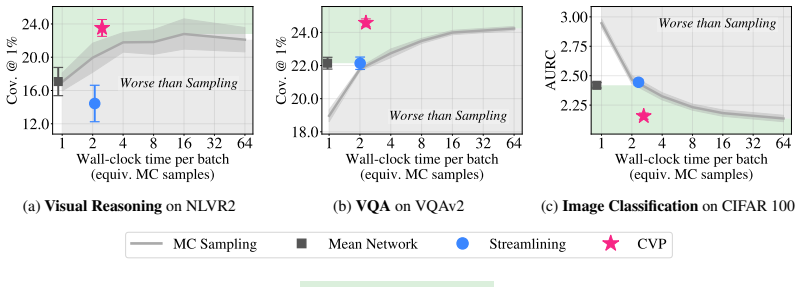
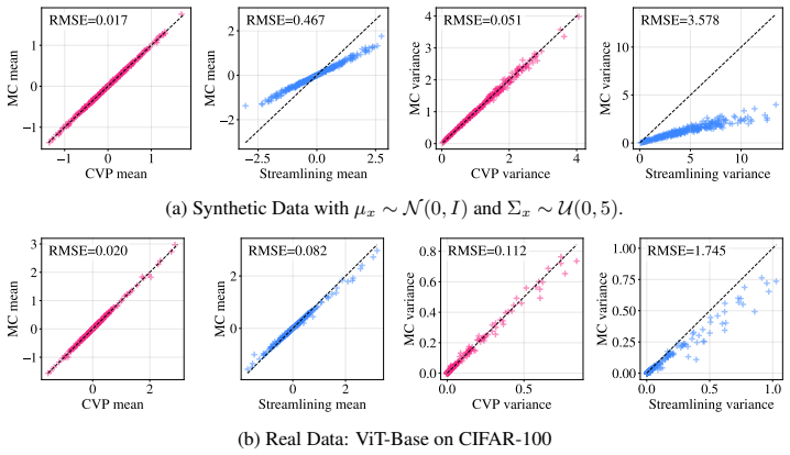
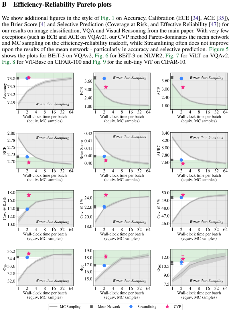
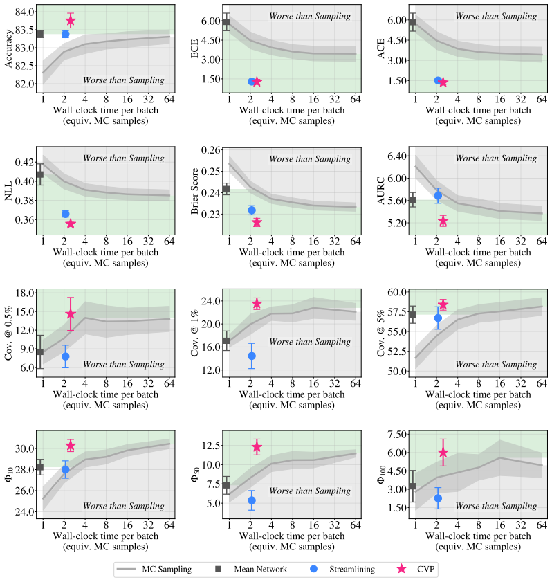
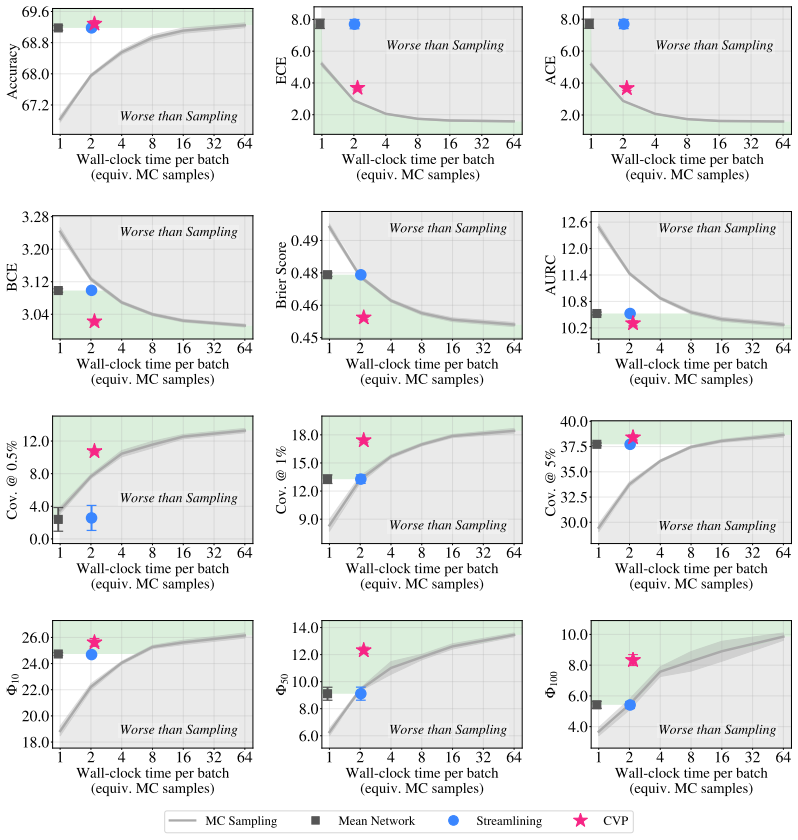
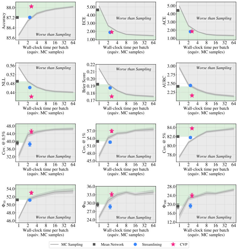
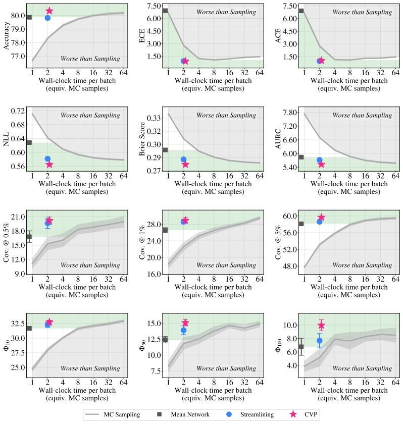
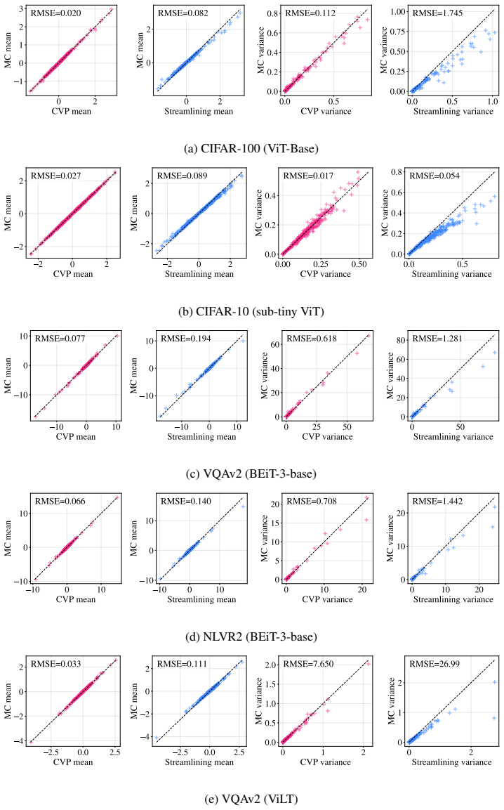
We propose Calibrated Variance Propagation (CVP), which introduces a new propagation method for normalization layers, combines it with recent techniques for handling activation functions, and absorbs residual error through a light calibration step. CVP yields comparably accurate uncertainty estimates to MC sampling across transformers and CNNs, at a fraction of the cost. Against prior variance propagation work, CVP improves coverage at 0.5% risk from 8.2% to 14.6% with BEiT-3 on NLVR2 and from 2.6% to 10.8% with ViLT on VQAv2, with gains extending to convolutional architectures.
What carries the argument
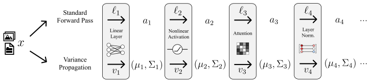
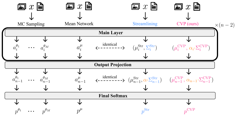
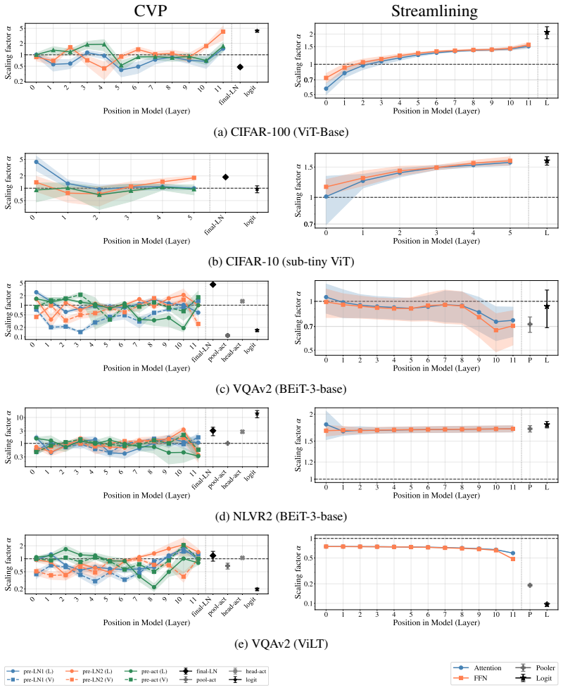
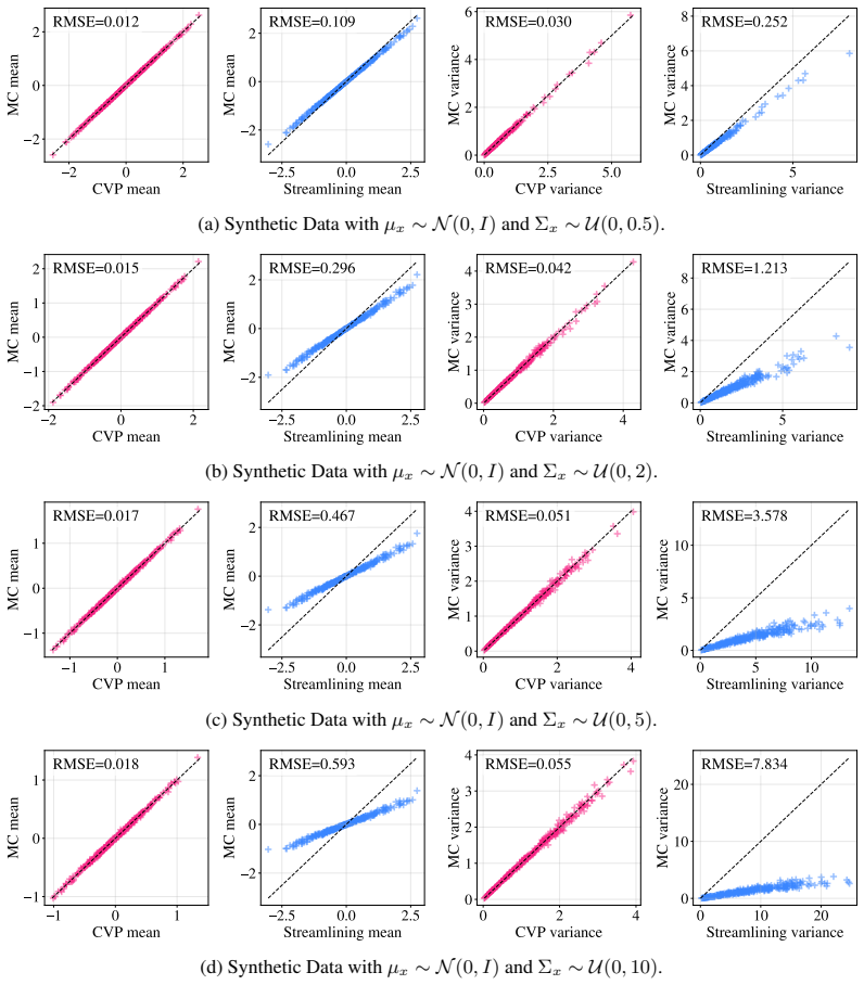
Calibrated Variance Propagation (CVP): layer-wise analytical variance approximation extended to normalization layers and activations, followed by a light calibration step to correct residuals.
Load-bearing premise
The light calibration step can absorb residual approximation error from the layer-wise propagation rules without introducing new bias or requiring task-specific retuning.
What would settle it
A new test on an unseen architecture where CVP coverage at 0.5% risk remains below Monte Carlo sampling levels after calibration would falsify the claim of comparable accuracy.
Figures
read the original abstract
Modern deep learning models remain notoriously prone to overconfidence, limiting their reliability in high-stakes applications. Bayesian methods aim to counter this by learning a distribution over model parameters, and recent advances now make this feasible for large-scale architectures at costs comparable to AdamW. However, a challenge remains at test time: predictions must be averaged across many forward passes with weights sampled from the posterior, which is prohibitively expensive. Variance propagation offers an efficient alternative, computing layer-wise analytical approximations of uncertainty in a single forward pass. While such techniques are effective for MLPs, their extension to modern architectures remains challenging, due to increased depth and diversity of layer types. To fill this gap, we propose Calibrated Variance Propagation (CVP), which introduces a new propagation method for normalization layers, combines it with recent techniques for handling activation functions, and absorbs residual error through a light calibration step. CVP yields comparably accurate uncertainty estimates to MC sampling across transformers and CNNs, at a fraction of the cost. Against prior variance propagation work, CVP improves coverage at $0.5\%$ risk from $8.2\%$ to $14.6\%$ with BEiT-3 on Visual Reasoning (NLVR2) and from $2.6\%$ to $10.8\%$ with ViLT on VQAv2, with gains extending to convolutional architectures.
Editorial analysis
A structured set of objections, weighed in public.
Referee Report
Summary. The paper proposes Calibrated Variance Propagation (CVP) as a sampling-free method for uncertainty estimation in Bayesian deep learning. It develops new analytical propagation rules for normalization layers, integrates recent techniques for activation functions, and applies a light calibration step to correct residual approximation errors from the layer-wise rules. CVP is claimed to match the accuracy of Monte Carlo sampling across transformers (e.g., BEiT-3, ViLT) and CNNs at far lower cost, with reported coverage gains at 0.5% risk level from 8.2% to 14.6% on NLVR2 and from 2.6% to 10.8% on VQAv2 versus prior variance propagation baselines.
Significance. If the central claims hold without hidden task-specific overhead, CVP would provide a practical, single-pass alternative to sampling-based Bayesian inference for large-scale models, addressing a key barrier to reliable uncertainty quantification in transformers and CNNs. The explicit coverage improvements over prior propagation methods and the focus on modern architectures represent a meaningful incremental advance if the calibration step proves general.
major comments (2)
- [Method section on calibration] The calibration step (described in the method section following the propagation rules) is load-bearing for the central claim that CVP remains sampling-free and general. The manuscript must demonstrate that the calibration parameters are fitted once per architecture (or globally) rather than per-task, per-dataset, or per-risk-level; otherwise the reported coverage gains could be artifacts of fitting rather than intrinsic propagation accuracy, directly engaging the skeptic concern about reintroducing task-dependent overhead.
- [Propagation rules section] § on normalization propagation and activation handling: the new rules are presented as analytical approximations, but no derivation details, error bounds, or ablation isolating the contribution of each rule versus the calibration correction are provided. This leaves open whether the coverage improvements reduce to the calibration parameters themselves.
minor comments (2)
- [Abstract] Abstract reports specific coverage numbers without referencing the corresponding tables or figures in the main text; add explicit cross-references.
- [Method] Notation for variance propagation through normalization layers should be clarified with an explicit equation for the mean and variance updates to aid reproducibility.
Simulated Author's Rebuttal
We thank the referee for the constructive feedback and the recommendation for major revision. We address each major comment below, clarifying the calibration procedure and committing to additional details and ablations on the propagation rules.
read point-by-point responses
-
Referee: [Method section on calibration] The calibration step (described in the method section following the propagation rules) is load-bearing for the central claim that CVP remains sampling-free and general. The manuscript must demonstrate that the calibration parameters are fitted once per architecture (or globally) rather than per-task, per-dataset, or per-risk-level; otherwise the reported coverage gains could be artifacts of fitting rather than intrinsic propagation accuracy, directly engaging the skeptic concern about reintroducing task-dependent overhead.
Authors: We agree this demonstration is essential to support the sampling-free claim. In our experiments the calibration parameters are fitted once per architecture on a small held-out validation split drawn from the pre-training distribution and then held fixed across downstream tasks and risk levels (e.g., the identical parameters are used for BEiT-3 on both NLVR2 and VQAv2). We will revise the method section to state this procedure explicitly, add a table reporting the calibration data size and fitting protocol, and include an ablation confirming that per-architecture parameters generalize without per-task or per-dataset refitting. This revision will be made. revision: yes
-
Referee: [Propagation rules section] § on normalization propagation and activation handling: the new rules are presented as analytical approximations, but no derivation details, error bounds, or ablation isolating the contribution of each rule versus the calibration correction are provided. This leaves open whether the coverage improvements reduce to the calibration parameters themselves.
Authors: We accept that the current presentation lacks sufficient transparency. We will add a supplementary section containing the full derivations of the normalization-layer moment-matching rules, the assumptions involved, and a numerical error analysis on synthetic layer compositions. We will also insert an ablation that replaces our new normalization rules with standard variance propagation while keeping the calibration step fixed, thereby isolating the incremental benefit of the new rules. These additions will appear in the revised manuscript. revision: yes
Circularity Check
No significant circularity; derivation rests on new propagation rules plus light calibration
full rationale
The paper proposes new layer-wise variance propagation rules for normalization layers, combines them with existing activation handling techniques, and applies a light calibration step to absorb residual approximation error. No equations or descriptions in the provided text show that the final uncertainty estimates or coverage metrics are defined in terms of the calibration parameters by construction, nor that any 'prediction' reduces to a fitted input. The reported improvements (e.g., coverage gains on BEiT-3 and ViLT) are attributed to the propagation method itself rather than tautological fitting. The method is presented as self-contained against MC sampling baselines, with the calibration described as a minor post-processing step that does not undermine the sampling-free claim. No self-citation chains or uniqueness theorems are invoked in a load-bearing way within the abstract or reader's summary.
Axiom & Free-Parameter Ledger
free parameters (1)
- calibration parameters
axioms (1)
- domain assumption Analytical variance propagation through normalization layers can be defined without introducing significant bias relative to Monte Carlo sampling.
Reference graph
Works this paper leans on
-
[1]
L. J. Ba, J. R. Kiros, and G. E. Hinton. Layer Normalization.arXiv preprint arXiv:1607.06450, 2016
Pith/arXiv arXiv 2016
-
[2]
C. M. Bishop.Pattern Recognition and Machine Learning. Information Science and Statistics. Springer, New York, NY , 2006
2006
-
[3]
Blundell, J
C. Blundell, J. Cornebise, K. Kavukcuoglu, and D. Wierstra. Weight Uncertainty in Neural Network. In F. R. Bach and D. M. Blei, editors,International Conference on Machine Learning (ICML), 2015
2015
-
[4]
G. W. Brier. Verification of Forecasts Expressed in Terms of Probability.Monthly Weather Review, 78(1):1–3, 1950
1950
-
[5]
H. Chen. Improving Audio Question Answering with Variational Inference.arXiv preprint arXiv:2601.12700, 2026
arXiv 2026
-
[6]
C. K. Chow. On optimum recognition error and reject tradeoff.IEEE Trans. Inf. Theory, 16(1): 41–46, 1970
1970
-
[7]
M. Dahl, V . Magesh, M. Suzgun, and D. E. Ho. Large Legal Fictions: Profiling Legal Halluci- nations in Large Language Models.Journal of Legal Analysis, 16(1):64–93, 2024
2024
-
[8]
J. Daunizeau. Semi-analytical approximations to statistical moments of sigmoid and softmax mappings of normal variables.arXiv preprint arXiv:1703.00091, 2017
Pith/arXiv arXiv 2017
-
[9]
Dosovitskiy, L
A. Dosovitskiy, L. Beyer, A. Kolesnikov, D. Weissenborn, X. Zhai, T. Unterthiner, M. Dehghani, M. Minderer, G. Heigold, S. Gelly, J. Uszkoreit, and N. Houlsby. An Image is Worth 16x16 Words: Transformers for Image Recognition at Scale. InInternational Conference on Learning Representations (ICLR), 2021
2021
-
[10]
El-Yaniv and Y
R. El-Yaniv and Y . Wiener. On the Foundations of Noise-Free Selective Classification.J. Mach. Learn. Res. (JMLR), 11:1605–1641, 2010
2010
-
[11]
A. Y . K. Foong, D. R. Burt, Y . Li, and R. E. Turner. On the Expressiveness of Approximate Inference in Bayesian Neural Networks. InAdvances in Neural Information Processing Systems (NeurIPS), 2020
2020
-
[12]
B. J. Frey and G. E. Hinton. Variational Learning in nonlinear Gaussian belief networks.Neural Computation, 11(1):193–213, 1999
1999
-
[13]
Gal and Z
Y . Gal and Z. Ghahramani. Dropout as a Bayesian Approximation: Representing Model Uncertainty in Deep Learning. InInternational Conference on Machine Learning (ICML), 2016
2016
-
[14]
Gast and S
J. Gast and S. Roth. Lightweight Probabilistic Deep Networks. InIEEE/CVF Conference on Computer Vision and Pattern Recognition (CVPR), 2018
2018
-
[15]
Geifman and R
Y . Geifman and R. El-Yaniv. Selective Classification for Deep Neural Networks. InAdvances in Neural Information Processing Systems (NeurIPS), 2017. 10
2017
-
[16]
Goyal, T
Y . Goyal, T. Khot, D. Summers-Stay, D. Batra, and D. Parikh. Making the V in VQA Matter: Elevating the Role of Image Understanding in Visual Question Answering. InIEEE/CVF Conference on Computer Vision and Pattern Recognition (CVPR), 2017
2017
-
[17]
A. Graves. Practical Variational Inference for Neural Networks. InAdvances in Neural Information Processing Systems (NeurIPS), 2011
2011
-
[18]
C. Guo, G. Pleiss, Y . Sun, and K. Q. Weinberger. On Calibration of Modern Neural Networks. In D. Precup and Y . W. Teh, editors,International Conference on Machine Learning (ICML), 2017
2017
-
[19]
Gurari, Q
D. Gurari, Q. Li, A. J. Stangl, A. Guo, C. Lin, K. Grauman, J. Luo, and J. P. Bigham. VizWiz Grand Challenge: Answering Visual Questions from Blind People. InIEEE/CVF Conference on Computer Vision and Pattern Recognition (CVPR), 2018
2018
-
[20]
J. M. Hernández-Lobato and R. P. Adams. Probabilistic Backpropagation for Scalable Learning of Bayesian Neural Networks. InInternational Conference on Machine Learning (ICML), 2015
2015
-
[21]
Hobbhahn, A
M. Hobbhahn, A. Kristiadi, and P. Hennig. Fast predictive uncertainty for classification with Bayesian deep networks. InConference on Uncertainty in Artificial Intelligence (UAI), 2022
2022
-
[22]
Ioffe and C
S. Ioffe and C. Szegedy. Batch Normalization: Accelerating Deep Network Training by Reducing Internal Covariate Shift. In F. R. Bach and D. M. Blei, editors,International Conference on Machine Learning (ICML), 2015
2015
-
[23]
A. T. Kalai, O. Nachum, S. S. Vempala, and E. Zhang. Why Language Models Hallucinate. arXiv preprint arXiv:2509.04664, 2025
Pith/arXiv arXiv 2025
-
[24]
W. Kim, B. Son, and I. Kim. ViLT: Vision-and-Language Transformer Without Convolution or Region Supervision. In M. Meila and T. Zhang, editors,International Conference on Machine Learning (ICML), 2021
2021
-
[25]
Kirichenko, M
P. Kirichenko, M. Ibrahim, K. Chaudhuri, and S. Bell. AbstentionBench: Reasoning LLMs Fail on Unanswerable Questions. InAdvances in Neural Information Processing Systems (NeurIPS) Datasets and Benchmarks Track, 2025
2025
-
[26]
Krizhevsky, G
A. Krizhevsky, G. Hinton, et al. Learning multiple layers of features from tiny images. 2009
2009
-
[27]
S. Kuang and X. Lin. Exact closed-form Gaussian moments of residual layers.arXiv preprint arXiv:2601.22307, 2026
Pith/arXiv arXiv 2026
-
[28]
Lakshminarayanan, A
B. Lakshminarayanan, A. Pritzel, and C. Blundell. Simple and Scalable Predictive Uncertainty Estimation using Deep Ensembles. InAdvances in Neural Information Processing Systems (NeurIPS), 2017
2017
-
[29]
Leibig, V
C. Leibig, V . Allken, M. S. Ayhan, P. Berens, and S. Wahl. Leveraging uncertainty information from deep neural networks for disease detection.Scientific Reports, 7(1):17816, 2017
2017
-
[30]
R. Li, M. Klasson, A. Solin, and M. Trapp. Streamlining Prediction in Bayesian Deep Learning. InInternational Conference on Learning Representations (ICLR), 2025
2025
-
[31]
Z. Lu, E. Ie, and F. Sha. Mean-Field Approximation to Gaussian-Softmax Integral with Application to Uncertainty Estimation.arXiv preprint arXiv:2006.07584, 2021
arXiv 2006
-
[32]
W. J. Maddox, P. Izmailov, T. Garipov, D. P. Vetrov, and A. G. Wilson. A Simple Baseline for Bayesian Uncertainty in Deep Learning. InAdvances in Neural Information Processing Systems (NeurIPS), 2019
2019
-
[33]
Monchot, L
P. Monchot, L. Coquelin, S. J. Petit, S. Marmin, E. L. Pennec, and N. Fischer. Input uncertainty propagation through trained neural networks. InInternational Conference on Machine Learning (ICML), 2023
2023
-
[34]
M. P. Naeini, G. F. Cooper, and M. Hauskrecht. Obtaining Well Calibrated Probabilities Using Bayesian Binning. InAAAI Conference on Artificial Intelligence (AAAI), 2015. 11
2015
-
[35]
Nixon, M
J. Nixon, M. W. Dusenberry, L. Zhang, G. Jerfel, and D. Tran. Measuring Calibration in Deep Learning. InIEEE/CVF Conference on Computer Vision and Pattern Recognition (CVPR), 2019
2019
-
[36]
Osawa, S
K. Osawa, S. Swaroop, M. E. Khan, A. Jain, R. Eschenhagen, R. E. Turner, and R. Yokota. Prac- tical Deep Learning with Bayesian Principles. InAdvances in Neural Information Processing Systems (NeurIPS), 2019
2019
-
[37]
Petersen, A
F. Petersen, A. A. Mishra, H. Kuehne, C. Borgelt, O. Deussen, and M. Yurochkin. Uncertainty Quantification via Stable Distribution Propagation. InInternational Conference on Learning Representations (ICLR), 2024
2024
-
[38]
Postels, F
J. Postels, F. Ferroni, H. Coskun, N. Navab, and F. Tombari. Sampling-Free Epistemic Uncer- tainty Estimation Using Approximated Variance Propagation. InInternational Conference on Computer Vision (ICCV), 2019
2019
-
[39]
Radford, J
A. Radford, J. Wu, R. Child, D. Luan, D. Amodei, I. Sutskever, et al. Language Models are Unsupervised Multitask Learners.OpenAI blog, 1(8):9, 2019
2019
-
[40]
Radford, J
A. Radford, J. W. Kim, C. Hallacy, A. Ramesh, G. Goh, S. Agarwal, G. Sastry, A. Askell, P. Mishkin, J. Clark, G. Krueger, and I. Sutskever. Learning Transferable Visual Models From Natural Language Supervision. InInternational Conference on Machine Learning (ICML), pages 8748–8763, 2021
2021
-
[41]
Y . Shen, N. Daheim, B. Cong, P. Nickl, G. M. Marconi, C. Bazan, R. Yokota, I. Gurevych, D. Cremers, M. E. Khan, and T. Möllenhoff. Variational Learning is Effective for Large Deep Networks. InInternational Conference on Machine Learning (ICML), 2024
2024
-
[42]
Singh and S
S. Singh and S. Krishnan. Filter Response Normalization Layer: Eliminating Batch Dependence in the Training of Deep Neural Networks. InIEEE/CVF Conference on Computer Vision and Pattern Recognition (CVPR), 2020
2020
-
[43]
A. Suhr, S. Zhou, A. Zhang, I. Zhang, H. Bai, and Y . Artzi. A Corpus for Reasoning about Natu- ral Language Grounded in Photographs. InAnnual Meeting of the Association for Computational Linguistics (ACL), 2019
2019
-
[44]
B. Trippe and R. Turner. Overpruning in Variational Bayesian Neural Networks.arXiv preprint arXiv:1801.06230, 2018
Pith/arXiv arXiv 2018
-
[45]
Vaswani, N
A. Vaswani, N. Shazeer, N. Parmar, J. Uszkoreit, L. Jones, A. N. Gomez, L. Kaiser, and I. Polosukhin. Attention is All you Need. InAdvances in Neural Information Processing Systems (NeurIPS), 2017
2017
-
[46]
W. Wang, H. Bao, L. Dong, J. Bjorck, Z. Peng, Q. Liu, K. Aggarwal, O. K. Mohammed, S. Singhal, S. Som, and F. Wei. Image as a Foreign Language: BEIT Pretraining for Vision and Vision-Language Tasks. InIEEE/CVF Conference on Computer Vision and Pattern Recognition (CVPR), 2023
2023
-
[47]
Whitehead, S
S. Whitehead, S. Petryk, V . Shakib, J. Gonzalez, T. Darrell, A. Rohrbach, and M. Rohrbach. Reliable Visual Question Answering: Abstain Rather Than Answer Incorrectly. InEuropean Conference on Computer Vision (ECCV), 2022
2022
-
[48]
T. J. Wieczorek, N. Daun, M. E. Khan, and M. Rohrbach. Variational Visual Question Answering for Uncertainty-Aware Selective Prediction.Trans. Mach. Learn. Res. (TMLR), 2026. URL https://openreview.net/forum?id=jtnMIbJIso
2026
-
[49]
Wright, Y
O. Wright, Y . Nakahira, and J. M. Moura. An Analytic Solution to Covariance Propagation in Neural Networks. InInternational Conference on Artificial Intelligence and Statistics (AISTATS), 2024
2024
-
[50]
A. Wu, S. Nowozin, E. Meeds, R. E. Turner, J. M. Hernández-Lobato, and A. L. Gaunt. Deterministic Variational Inference for Robust Bayesian Neural Networks. InInternational Conference on Learning Representations (ICLR), 2019
2019
-
[51]
Zhang and Y
B. Zhang and Y . C. Shin. An adaptive Gaussian mixture method for nonlinear uncertainty propagation in neural networks.Neurocomputing, 458:170–183, 2021. 12 A Full derivations of Variance Propagation rules A.1 Notation and Prerequisites Throughout the derivations below, we make use of the following well-known results. Letα, αi, β∈R be constants and letX, ...
2021
-
[52]
Linearity of expectation: E "X i αiXi +β # = X i αi E[Xi] +β(I)
-
[53]
Expectation of products ofindependentvariables: E "Y i Xi # = Y i E[Xi](II)
-
[54]
Variance–expectation relation: Var[X] =E[X 2]−E[X] 2 (III)
-
[55]
Variance scaling: Var[αX+β] =α 2 Var[X](IV)
-
[56]
(III) to (V) additionally require finite second moments, and Eqs
Variance of sums ofindependentvariables: Var "X i Xi # = X i Var[Xi](V) These statements require finite expectations of the Xi; Eqs. (III) to (V) additionally require finite second moments, and Eqs. (II) and (V) require independence of theX i. We use the notation µz =E[z] for the mean, Σz = Var[z] for the variance, and σz = √Σz for the standard deviation....
-
[57]
sub-tiny
subsequently derived an exact closed form for Σy that avoids the series truncation, which we use throughout. We refer the reader to Appendix D of Kuang and Lin [27] for the full expression. A.4 Layer Normalization Recall the LayerNorm operation: given input activationsx∈R D, y= x−m(x)p s2(x) +ϵ ⊙γ+β,(19) where m(x) = 1 D P d xd and s2(x) = 1 D P d(xd −m(x...
discussion (0)
Sign in with ORCID, Apple, or X to comment. Anyone can read and Pith papers without signing in.