REVIEW 4 major objections 6 minor 20 references
Large Scale Evaluation of Deep Learning-based Explainable Solar Flare Forecasting Models with Attribution-based Proximity Analysis
T0 review · 4 major / 6 minor · reviewed 2026-08-12 · deepseek-v4-flash
Pith's one-line read This paper introduces an automated proximity-based framework, PEPS-SF, for scoring whether post hoc explanations of full-disk solar flare models point near active regions, and reports that one of two compared models sits substantially…
desk verdict A useful automated pipeline for checking explanation alignment to active regions, but the proximity metrics lack baselines and sensitivity analysis, so the M1/M2 comparison is not yet evidence of explanation quality. read the letter →
The pith
A machine-rendered reading of the paper's core claim, the machinery that carries it, and where it could break.
The reading
What carries the argument
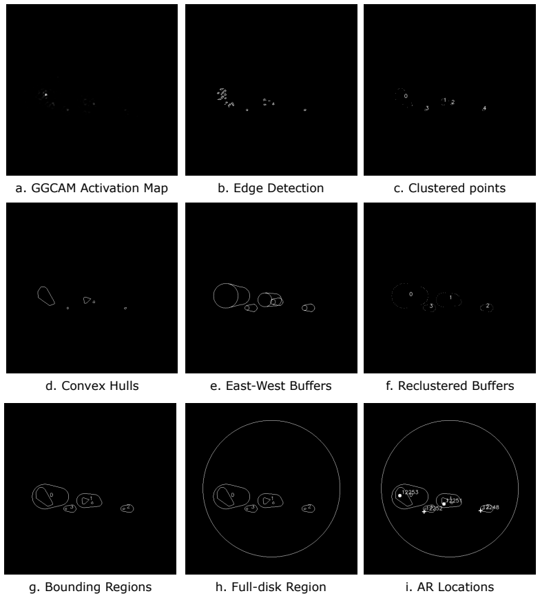
The load-bearing object is PEPS-SF, a proximity-based evaluation pipeline defined in Algorithm 1. It takes a magnetogram and the coordinates of active regions and flare locations, generates a Guided Grad-CAM attribution map, scales intensities to 0-255, applies Canny edge detection with thresholds 30 and 50, clusters edge pixels with DBSCAN using a minimum of 2 samples and a maximum distance of 10 pixels, derives convex hulls, pads them with a 5-pixel eastward and a 40-pixel westward buffer to account for solar rotation over the 24-hour window, merges nearby hulls, masks to the solar disk, and converts heliographic coordinates to pixel coordinates. The two output metrics are the Proximity Score, the mean minimum Euclidean distance from each active region to the nearest buffered hull, and the Attribution Colocation Ratio, the fraction of active regions inside those bounding regions. These metrics carry the argument because the entire comparison of M1 and M2 reduces to the numbers they produce.
What would settle it
Replace the real Guided Grad-CAM attribution maps with randomly placed hulls of matched size and run the same PEPS-SF pipeline; if the randomized hulls achieve an average Proximity Score at or below M2's 29.4 pixels or an Attribution Colocation Ratio near 0.55, then the metrics are rewarding diffuse coverage rather than explanation fidelity.
Extended reading notes
Core claim
The paper's central claim is that the reliability of post hoc explanations in solar flare forecasting can be scored automatically once the regions of interest, namely NOAA active regions and flare locations, are known. To that end it defines two metrics. The Proximity Score is the average Euclidean distance between each active region and the closest buffered convex hull built from the model's Guided Grad-CAM attribution map; a lower score means the explanation highlights pixels nearer the physically relevant region. The Attribution Colocation Ratio is the percentage of active regions that fall inside those buffered bounding regions. Applied to 5,923 full-disk magnetograms from 2020 to 2023, the framework reports that M2 is closer on average (29.4 versus 61.4 pixels) and more consistent across the true-positive, false-positive, true-negative, and false-negative categories, while both models place only about 55 percent of active regions inside their attribution hulls. The conclusion drawn is that one model's explanations align better with active-region structure and that the framework is a step toward operational, automated evaluation of explanation fidelity.
Load-bearing premise
The load-bearing premise, stated in Section II.B and partly conceded in Section V's note on preprocessing noise, is that an explanation counts as good exactly when its highlighted hulls sit near NOAA active-region centroids, and that the hand-set Canny, DBSCAN, and buffer parameters do not alter the model ranking; if either condition fails, the M1-versus-M2 comparison does not measure explanation quality.
Editorial extensions
If this is right
- A forecasting model's explanations can be graded without human raters whenever known active-region locations are available, making routine audits of deployed flare models possible.
- M2's lower average Proximity Score (29.4 versus 61.4 pixels) is evidence that its Guided Grad-CAM explanations concentrate closer to active regions than M1's explanations do.
- An Attribution Colocation Ratio near 0.55 for both models means roughly 45 percent of active regions are not covered by the attribution hulls, so neither model's explanations fully account for all flaring regions in a given image.
- Because the Proximity Score is continuous and the Attribution Colocation Ratio is binary, they answer different audit questions: how far off is the explanation, and does it cover the region at all.
- Applied per prediction category, the framework can flag systematic failures such as false negatives whose explanations point far from the actual active regions.
Reading between the lines
- A check the paper leaves implicit: replacing active-region centroids with the actual NOAA flare coordinates in Equation (4) could re-rank the models, since the stated fidelity target is the active region rather than the flare itself.
- The reported ordering is meaningful only if it is stable under preprocessing choices; a grid search over Canny thresholds, DBSCAN parameters, and buffer widths would show whether M2's 32-pixel advantage is robust or an artifact of a few parameter values.
- The same pipeline could be run on other attribution methods, such as Integrated Gradients or DeepLIFT, to rank explanation algorithms rather than models, turning Proximity Score and Attribution Colocation Ratio into general-purpose selection criteria.
- Without a baseline of randomized attribution hulls matched in size and location distribution, a low Proximity Score might reflect diffuse or centrally concentrated explanations rather than true alignment; adding such a baseline would establish significance.
Editorial analysis
A structured set of objections, weighed in public.
Referee Report
Summary. The paper proposes PEPS-SF, an automated framework for evaluating post hoc explanations in full-disk solar flare forecasting. The framework derives attribution maps with Guided Grad-CAM, processes them through edge detection, density-based clustering, convex hull extraction, buffering, and re-clustering, and then compares the resulting regions to NOAA active-region locations using two new metrics: Proximity Score (Eq. 4) and Attribution Colocation Ratio (Eq. 5). The method is applied to two previously published CNN models, M1 and M2, over a dataset of 5,923 full-disk magnetograms from 2020 to 2023. The paper reports that M2 has a lower average Proximity Score (29.4 vs. 61.4 pixels) while both models have similar ACR values (about 0.55), and it interprets this as evidence that M2's explanations are more accurately aligned with active regions. The contribution is framed as a fully automated, quantitative evaluation of explanation quality for operational use.
Significance. If the proximity metrics are valid measures of explanation quality, the framework would be a useful step toward automated interpretability evaluation in a high-stakes operational domain. The paper has real strengths: an explicitly specified algorithm, a large evaluation dataset, a concrete comparison between two models, and an open-source code repository. The fundamental validity of the metric, however, is not yet established. The paper provides no random or uniformity baseline, no validation against human judgments or alternative attribution methods, and no sensitivity analysis for the hand-set parameters. Because the Proximity Score has no specificity or coverage penalty, a trivial diffuse attribution map can achieve a perfect score, so the reported M1/M2 difference may reflect attribution breadth rather than localization quality. These issues are fixable with additional controls and analysis, but they currently prevent the central claim from being supported.
major comments (4)
- [Section II.B, Eqs. (4) and (5)] The Proximity Score is the average Euclidean distance from each active region to the closest attribution convex hull, with no penalty for attribution regions that cover large portions of the solar disk. A spatially diffuse attribution map that covers the full disk will have dmin = 0 for every AR, yielding PS = 0 and ACR = 1. The preprocessing pipeline actively enlarges regions through eastward/westward buffers and re-clustering (Fig. 3e-f), so the smaller average PS of M2 in Table II (29.4 vs. 61.4) is indistinguishable from M2 having broader, less specific attribution maps. The paper reports no measure of attribution spread or coverage, so the claim that lower PS reflects more accurate localization is not established.
- [Section II.B and Table I] The central assumption that proximity of attribution hulls to NOAA active-region centroids is a valid proxy for explanation quality is introduced without validation. The manuscript gives no random or uniform-attribution baseline, no comparison with human judgments (despite the prior human-in-the-loop evaluation in [6]), and no comparison with alternative attribution methods such as Integrated Gradients or DeepLIFT. A minimal control would be to run the same PEPS-SF pipeline on random or uniform attribution maps and on a second attribution method; if those baselines produce similar PS/ACR values to the real models, the metric would not be informative about explanation quality. Without such controls, the abstract's claim that the framework 'quantitatively assesses the accuracy and relevance' of explanations is unsupported.
- [Section IV.A, Table III] The conclusion that M2 is 'more accurate and consistent' than M1 is based on raw mean and standard deviation values, but no statistical tests or confidence intervals are provided. The standard deviations are very large relative to the mean differences (e.g., FN: 72.49 vs. 38.02 with SDs 71.89 and 46.96; TP: 59.43 vs. 52.03 with SDs 68.05 and 48.68), so the reported differences may not be statistically significant. Since the four contingency categories are not independent across images, a paired bootstrap or permutation test over the 5,923 images is needed to support the comparative claims.
- [Section III, Table I] The six hand-set parameters (Canny thresholds 30 and 50, DBSCAN min_samples 2 and max_dist 10, eastward buffer 5, and westward buffer 40) are used without any sensitivity analysis. Because these parameters control the merging and enlargement of attribution regions, the relative ordering of M1 and M2 in Table II could change over plausible parameter ranges. The authors should vary each parameter over a reasonable grid and report whether the qualitative comparison is stable. Without this analysis, the reported M1/M2 difference cannot be distinguished from an artifact of the particular parameter values chosen.
minor comments (6)
- [Abstract and Section II.B] The wording 'quantitatively assesses the accuracy and relevance of local explanations' overstates what the geometric metrics measure; consider replacing 'accuracy and relevance' with 'spatial alignment' until the proxy is validated.
- [Figure 2 caption] The caption contains the phrase 'An schematic overview'; it should read 'A schematic overview'.
- [Section II.A] The sentence 'In Step (a) , the Guided-GradCAM image is resized...' contains an awkward space before the comma and inconsistent naming (Guided-GradCAM vs. GGCAM); please standardize the terminology.
- [Eq. (5) and Table II] Equation (5) defines ACR as a percentage by multiplying by 100, but Table II reports values such as 0.552943 without a percent sign; clarify the units and formatting consistently.
- [Section IV.A] The text states that M2 'outperforms M1 in false negatives, false positives, and true negatives,' but Table III shows FP means of 52.95 (M1) and 55.63 (M2), so M1 has the lower FP score; the sentence should be corrected to match the table.
- [Section IV.B] The text states that M1 'generally exhibits higher mean ACRs across most categories,' but Table IV shows FN ACR of 0.514 for M1 and 0.521 for M2, so the claim needs qualification or correction.
Circularity Check
No circular derivation: PS/ACR are direct distance measurements against external NOAA active-region coordinates, and the M1/M2 comparison is empirical; validity concerns about the proximity proxy are not circularity.
full rationale
The paper's derivation chain is the PEPS-SF algorithm: Guided Grad-CAM attribution maps, Canny edge detection, DBSCAN clustering, convex hulls, buffering, and Euclidean distances to NOAA active-region coordinates. None of these quantities is fitted to the target conclusion. Active-region coordinates come from an external NOAA database, Guided Grad-CAM is a standard external attribution method, and the two CNN models M1 and M2 are taken from prior work only as test objects, not as evidence for the metric. The headline result—that M2 has a lower average Proximity Score (29.4 vs 61.4 pixels)—is a direct empirical measurement using Eq. (4), not a quantity implied by the definition of the inputs. The Attribution Colocation Ratio similarly is an empirical count using Eq. (5). The main weakness, that the Proximity Score rewards diffuse over-coverage and that 'explanation quality' is operationalized as proximity to active regions without validation against human judgments or random baselines, is a validity and correctness concern, not a circularity. The paper contains many self-citations to prior model papers, but these are contextual references to the models being evaluated; no load-bearing argument reduces to a self-citation chain or to a uniqueness theorem imported from the authors. The comparison between M1 and M2 remains an independent measurement against external data. Therefore no significant circularity is present.
Assumptions & free parameters
free parameters (6)
- Canny lower threshold =
30
- Canny upper threshold =
50
- DBSCAN min_samples =
2
- DBSCAN max distance (eps) =
10
- Eastward buffer =
5
- Westward buffer =
40
assumptions (6)
- standard math Euclidean distance, Canny edge detection, DBSCAN, and convex hull algorithms are correct and appropriate for the data
- domain assumption NOAA active region and flare databases are accurate and complete
- domain assumption Helioprojective-Cartesian to pixel conversion via Eq. (1)-(2) is valid for the full-disk magnetograms
- domain assumption Models M1 and M2 trained on 2010-2018 data can be meaningfully evaluated on 2020-2023 magnetograms
- ad hoc to paper Proximity of attribution hulls to AR centroids is a valid proxy for explanation quality
- ad hoc to paper Buffer widths of 5 and 40 pixels adequately account for solar rotation and evolution over the 24h prediction window
Cite this review
Pith. "Pith review of Large Scale Evaluation of Deep Learning-based Explainable Solar Flare Forecasting Models with Attribution-based Proximity Analysis." pith.science (2026). https://pith.science/paper/LIUNFSCL
@misc{pith2026241118070,
  author       = {Pith},
  title        = {Pith review of: Large Scale Evaluation of Deep Learning-based Explainable Solar Flare Forecasting Models with Attribution-based Proximity Analysis},
  year         = {2026},
  howpublished = {\url{https://pith.science/paper/LIUNFSCL}},
  note         = {Machine review of arXiv:2411.18070}
}
abstract
Accurate and reliable predictions of solar flares are essential due to their potentially significant impact on Earth and space-based infrastructure. Although deep learning models have shown notable predictive capabilities in this domain, current evaluations often focus on accuracy while neglecting interpretability and reliability--factors that are especially critical in operational settings. To address this gap, we propose a novel proximity-based framework for analyzing post hoc explanations to assess the interpretability of deep learning models for solar flare prediction. Our study compares two models trained on full-disk line-of-sight (LoS) magnetogram images to predict $\geq$M-class solar flares within a 24-hour window. We employ the Guided Gradient-weighted Class Activation Mapping (Guided Grad-CAM) method to generate attribution maps from these models, which we then analyze to gain insights into their decision-making processes. To support the evaluation of explanations in operational systems, we introduce a proximity-based metric that quantitatively assesses the accuracy and relevance of local explanations when regions of interest are known. Our findings indicate that the models' predictions align with active region characteristics to varying degrees, offering valuable insights into their behavior. This framework enhances the evaluation of model interpretability in solar flare forecasting and supports the development of more transparent and reliable operational systems.
Figures


Figures from the paper (2 more)


Reference graph
Works this paper leans on
-
[6]
C. Pandey, A. Ji, T. Nandakumar, R. A. Angryk, and B. Aydin, “Ex- ploring deep learning for full-disk solar flare prediction with empirical insights from guided grad-cam explanations,” 2023
work page 2023
-
[1]
An observational overview of solar flares,
L. Fletcher, B. R. Dennis, H. S. Hudson, S. Krucker, K. Phillips, A. Veronig, M. Battaglia, L. Bone, A. Caspi, Q. Chen, P. Gallagher, P. T. Grigis, H. Ji, W. Liu, R. O. Milligan, and M. Temmer, “An observational overview of solar flares,” Space Science Reviews , vol. 159, no. 1, pp. 19–106, Aug. 2011
work page 2011
-
[2]
Y . Yasyukevich, E. Astafyeva, A. Padokhin, V . Ivanova, S. Syrovatskii, and A. Podlesnyi, “The 6 september 2017 x-class solar flares and their impacts on the ionosphere, gnss, and hf radio wave propagation,” Space Weather, vol. 16, Jul. 2018
work page 2017
-
[3]
Flare-productive active regions,
S. Toriumi and H. Wang, “Flare-productive active regions,” Living Reviews in Solar Physics , vol. 16, no. 1, p. 3, May 2019
work page 2019
-
[4]
Solar flare forecasting with deep neural networks using compressed full-disk hmi magnetograms,
C. Pandey, R. Angryk, and B. Aydin, “Solar flare forecasting with deep neural networks using compressed full-disk hmi magnetograms,” in2021 IEEE International Conference on Big Data (Big Data), 2021, pp. 1725– 1730
work page 2021
-
[5]
C. Pandey, A. Ji, R. A. Angryk, M. K. Georgoulis, and B. Aydin, “Towards coupling full-disk and active region-based flare prediction for operational space weather forecasting,” Frontiers in Astronomy and Space Sciences, vol. 9, Aug. 2022
work page 2022
-
[7]
Grad-cam: Visual explanations from deep networks via gradient-based localization,
R. R. Selvaraju, M. Cogswell, A. Das, R. Vedantam, D. Parikh, and D. Batra, “Grad-cam: Visual explanations from deep networks via gradient-based localization,” in 2017 IEEE International Conference on Computer Vision (ICCV) , 2017, pp. 618–626
work page 2017
-
[8]
Striving for simplicity: The all convolutional net,
J. T. Springenberg, A. Dosovitskiy, T. Brox, and M. Riedmiller, “Striving for simplicity: The all convolutional net,” 2014
work page 2014
Show all 20 references
-
[9]
Axiomatic attribution for deep networks,
M. Sundararajan, A. Taly, and Q. Yan, “Axiomatic attribution for deep networks,” 2017
2017
-
[10]
A unified approach to interpreting model predictions,
S. M. Lundberg and S.-I. Lee, “A unified approach to interpreting model predictions,” in Proceedings of the 31st International Conference on Neural Information Processing Systems , ser. NIPS’17. Red Hook, NY , USA: Curran Associates Inc., 2017, p. 4768–4777
2017
-
[11]
Supervised convolutional neural networks for classification of flaring and nonflaring active regions using line-of-sight magnetograms,
S. Bhattacharjee, R. Alshehhi, D. B. Dhuri, and S. M. Hanasoge, “Supervised convolutional neural networks for classification of flaring and nonflaring active regions using line-of-sight magnetograms,” Astro- physical Journal, vol. 898, no. 2, Aug. 2020
2020
-
[12]
Pandey, R
C. Pandey, R. A. Angryk, and B. Aydin, Explaining full-disk deep learning model for solar flare prediction using attribution methods . Springer Nature Switzerland, 2023, pp. 72–89
2023
-
[13]
Towards interpretable solar flare prediction with attention-based deep neural networks,
C. Pandey, A. Ji, R. A. Angryk, and B. Aydin, “Towards interpretable solar flare prediction with attention-based deep neural networks,” in 2023 IEEE Sixth International Conference on Artificial Intelligence and Knowledge Engineering (AIKE) , 2023, pp. 83–90
2023
-
[14]
Predicting solar flares using cnn and lstm on two solar cycles of active region data,
Z. S. et al., “Predicting solar flares using cnn and lstm on two solar cycles of active region data,” The Astrophysical Journal, vol. 931, no. 2, p. 163, 2022
2022
-
[15]
Learning important features through propagating activation differences,
A. Shrikumar, P. Greenside, and A. Kundaje, “Learning important features through propagating activation differences,” 2017
2017
-
[16]
Pandey, R
C. Pandey, R. A. Angryk, M. K. Georgoulis, and B. Aydin, Explainable deep learning-based solar flare prediction with post hoc attention for operational forecasting. Springer Nature Switzerland, 2023, pp. 567– 581
2023
-
[17]
Pandey, R
C. Pandey, R. A. Angryk, and B. Aydin, Deep neural networks based solar flare prediction using compressed full-disk line-of-sight magne- tograms. Springer International Publishing, 2022, pp. 380–396
2022
-
[18]
Unveiling the potential of deep learning models for solar flare prediction in near-limb regions,
C. Pandey, R. Angryk, and B. Aydin, “Unveiling the potential of deep learning models for solar flare prediction in near-limb regions,” in 2023 International Conference on Machine Learning and Applications (ICMLA), 2023, pp. 703–708
2023
-
[19]
Visual explanation of a deep learning solar flare forecast model and its relationship to physical parameters,
K. Yi, Y .-J. Moon, D. Lim, E. Park, and H. Lee, “Visual explanation of a deep learning solar flare forecast model and its relationship to physical parameters,” The Astrophysical Journal , vol. 910, no. 1, p. 8, 2021
2021
-
[20]
Attribution-based proximity analysis,
DMLAB, “Attribution-based proximity analysis,” 2024. [Online]. Avail- able: https://bitbucket.org/gsudmlab/solar-flare-prediction-evaluation/ src/main/
2024
Reviewed August 12, 2026 · model on record in the stance chip above.
Discussion (0). Continue with ORCID to comment.