DropoutTS: Sample-Adaptive Dropout for Robust Time Series Forecasting

Fei Wang; Qingsong Wen; Siru Zhong; Yiqiu Liu; Yuxuan Liang; Zezhi Shao; Zhiqing Cui

REVIEW 5 major objections 7 minor 1 cited by

A model-agnostic plug-in that sets each sample's dropout rate from its spectral noise score can make time series forecasters more accurate and more noise-resistant.

Reviewed by Pith at T0; open to challenge. T0 means a machine referee read the full paper against a public rubric. the ladder, T0–T4 →

Challenge this review Re-run · record.json Download PDF Read on arXiv ↗

T0 review · deepseek-v4-flash

2026-08-03 06:51 UTC pith:LP23IWK5

load-bearing objection A genuinely new sample-adaptive dropout mechanism with broad but thin empirical support; the noise-scoring interpretation needs validation against ground truth before the robustness story is secure. the 5 major comments →

arxiv 2601.21726 v2 pith:LP23IWK5 submitted 2026-01-29 cs.AI

DropoutTS: Sample-Adaptive Dropout for Robust Time Series Forecasting

Siru Zhong , Yiqiu Liu , Zhiqing Cui , Zezhi Shao , Fei Wang , Qingsong Wen , Yuxuan Liang This is my paper

classification cs.AI

keywords time series forecastingdropoutsample-adaptive regularizationspectral sparsitynoise quantificationspectral flatness measurestraight-through estimatorrobustness

verification ladder T0 review T1 audit T2 compute T3 formal T4 reserved

The pith

A machine-rendered reading of the paper's core claim, the machinery that carries it, and where it could break.

This paper tries to establish that the right amount of regularization for a time series sample can be read off the sample's own frequency spectrum. It introduces DropoutTS, a plug-in that scores how noisy each input window is by how poorly a learnable spectral filter can reconstruct it, then maps that score to a dropout rate: noisy samples get high dropout, clean samples get low dropout. The authors claim this works across six backbone architectures and seven real-world datasets plus a controlled synthetic benchmark, with large gains for noise-prone models (up to 46% MSE reduction) and no inference-time cost. If the claim holds, robustness to noise becomes a cheap, model-agnostic add-on rather than a data-pruning or probabilistic-modeling redesign.

Core claim

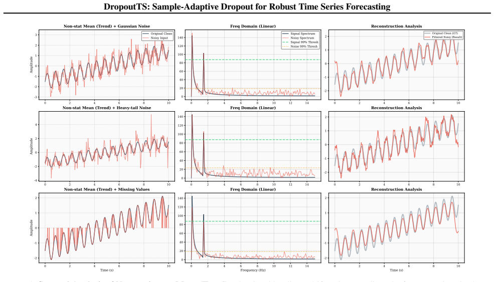
On the paper's own terms, the central claim is that spectral sparsity—the fact that valid temporal signals concentrate energy in a few dominant frequencies while noise spreads as a low broadband floor—gives a reliable, proxy-free per-instance noise metric. A learnable soft mask anchored to the Spectral Flatness Measure filters the spectrum; the mean absolute reconstruction residual becomes the noise score. Mapping that score through a batch-aware tanh/softplus curve to a dropout rate, and training the mask parameters end-to-end through a straight-through estimator, lets a backbone selectively suppress noisy samples while preserving clean ones. The result, the authors argue, is consistent acc

What carries the argument

Two coupled components carry the argument. The Spectral Noise Scorer detrends the input with global linear regression, takes log-normalized FFT amplitudes, filters them with a learnable soft threshold mask anchored to the Spectral Flatness Measure (which is near 0 for tonal signals and near 1 for white noise), and reconstructs the signal; the MAE of the residual is the per-sample noise score. The Sample-Adaptive Dropout module normalizes scores within a batch, maps them to a dropout probability p in [0.05, 0.5] via a learnable sensitivity curve, and generates a differentiable binary mask using the Straight-Through Estimator, allowing the task loss to backpropagate into the scorer parameters.

Load-bearing premise

The method assumes the per-sample noise score s (Eq. 7) measures true input noise rather than a learned proxy for sample difficulty; if s tracks hardness instead of noise, the robustness-by-noise story weakens, even if predictions still improve.

What would settle it

Instantiate the scorer on Synth-12 and compute the rank correlation between the predicted noise score s and the known injected noise level sigma (0.1 to 0.9). A weak, zero, or non-monotonic correlation would refute the claim that the spectral residual quantifies noise intensity.

Watch this falsifier — get emailed when new claim-graph text bears on it.

If this is right

DropoutTS can be added to existing forecasting backbones without changing their architecture or loss, with consistent gains reported across Transformer, CNN, and MLP models.
The 'fixed dropout paradox'—where static dropout both over-regularizes clean samples and under-regularizes noisy ones—would be resolved by sample-adaptive rates, explaining why fixed-rate dropout sometimes hurts.
Because the scorer is deactivated at inference, the robustness gains come with zero additional latency, making the method compatible with real-time forecasting.
The sparsity validation suggests that retaining roughly 10% of spectral coefficients is enough for high-fidelity reconstruction on real benchmarks, indicating a large noise floor in many standard datasets.
The method is complementary to data-centric selection: combining Selective Learning with DropoutTS reduces MSE further than either alone on the ILI dataset.

Where Pith is reading between the lines

These are editorial extensions of the paper, not claims the author makes directly.

If the noise score truly tracks synthetic ground-truth sigma, the same residual could be repurposed for other per-sample policies—sample weighting, curriculum pacing, or adaptive loss scaling—beyond dropout.
The reported negative correlation between Spectral Flatness Measure and estimated SNR (r about -0.85) suggests SFM could serve as a cheap, label-free data-quality diagnostic for forecasting datasets generally.
The gains concentrate on strongly periodic data (Weather, ETTh2), so a natural boundary to probe is whether sample-adaptive dropout helps on aperiodic, regime-switching series or on extremely short horizons, where spectral estimates are less stable.

Editorial analysis

A structured set of objections, weighed in public.

Desk editor's note, referee report, simulated authors' rebuttal, and a circularity audit.

Desk Editor's Note

A genuinely new sample-adaptive dropout mechanism with broad but thin empirical support; the noise-scoring interpretation needs validation against ground truth before the robustness story is secure.

read the letter

Worth your time. The core idea—per-sample dropout rates set by spectral reconstruction residuals via a learnable mask and a straight-through estimator—is new in the cited literature, and the paper shows it consistently helps, sometimes dramatically for weak backbones like Informer and modestly (0.5–2%) for strong ones like PatchTST and iTransformer. The design is clean, model-agnostic, and the code is available. That part holds up.

The soft spots are real but not fatal. First, there are no error bars or significance tests anywhere. Given the small gains on strong backbones, that matters: 1% MSE differences can easily be noise. Second, the comparison is against a single fixed dropout rate (p=0.1), not a tuned fixed dropout per backbone and dataset. Since the method's whole pitch is adaptivity, that undersells the baseline and weakens the claim. Third, and most important: the noise score s is trained end-to-end with the task loss through the STE path. The paper says the 'implicit feedback loop' drives clean samples to get lower dropout and noisy samples higher dropout. That means s is a learned proxy for whatever reduces forecasting loss—sample difficulty, maybe, or predictability—not necessarily input noise. The authors validate SFM against estimated SNR on real data, but they never check s against the known ground-truth σ in Synth-12. That validation is cheap and would directly support the 'noise quantification' narration. Without it, the mechanism could be doing generic sample reweighting, and the robustness interpretation is under-supported. The theory appendix is also coarse; a convexity argument plus a Rademacher bound that doesn't tightly follow from the model. I would not hang much on it.

That said, the central engineering claim—adaptive dropout helps—probably survives. The experiments are broad, the ablations are informative, and the efficiency analysis is a plus. This is a solid within-subfield contribution that needs a bit more rigor before the causal story is sold.

I would send this to peer review. The right referees can push for the Synth-12 ground-truth validation, tuned fixed-dropout baselines, and error bars. It is a paper worth engaging with, but I would advise any student reading it to treat the noise-scoring interpretation as an open question, not an established result.

Referee Report

5 major / 7 minor

Summary. DropoutTS is a model-agnostic plug-in that replaces fixed dropout in time series forecasters with a per-instance adaptive dropout rate. The rate is derived from a spectral noise score: the input is linearly detrended, transformed with FFT, filtered by a learnable soft mask anchored by the Spectral Flatness Measure, and the reconstruction residual (MAE) becomes the noise score. The score is normalized within a batch and mapped through a learned sensitivity curve to a dropout probability, with gradients flowing back through a straight-through estimator (Eq. 10). The authors evaluate the plug-in on six backbones (Informer, Crossformer, PatchTST, TimesNet, iTransformer, TimeMixer) over seven real-world datasets and a synthetic Synth-12 benchmark, reporting consistent MSE/MAE improvements, ablations, efficiency analysis, and a theoretical generalization bound in Appendix F.

Significance. If the central claims hold, DropoutTS would be a low-cost, architecture-agnostic robustness plug-in, and the 'capacity-centric modulation' frame would be a useful complement to data-pruning and prior-based robustness methods. The paper is commendable for releasing code, evaluating six diverse backbones, constructing a controllable synthetic benchmark with known noise levels, and including a compatibility study with Selective Learning. However, the currently reported evidence is not yet strong enough to support the 'universal robustness plugin' claim: there is no comparison against a tuned fixed dropout rate, no statistical uncertainty quantification, and the noise-scoring mechanism is not validated as measuring true input noise rather than sample difficulty.

major comments (5)

[§4.1–4.2, Eq. (7)–(11)] The noise score s is computed from a learnable spectral mask whose parameters (α, w_s, b_s, γ) are optimized end-to-end with the forecasting loss. The paper never validates s against the known ground-truth noise levels available in Synth-12 (σ ∈ {0.1,...,0.9}). Since σ is controlled, please report the per-sample correlation between s and σ (or SNR) in each noise regime, and compare with a purely difficulty-based proxy (e.g., loss of a fixed-threshold spectral residual). Without this test, the 'noise quantification' interpretation is not distinguished from generic sample reweighting, which is a load-bearing part of the contribution.
[§5.2, Tables 2 and 5] The superiority of the adaptive dropout over fixed dropout is not established. The ablation baseline uses a single fixed dropout rate p=0.1, and the Raw baselines in Tables 2–4 use the backbones' default hyperparameters. To support the 'sample-adaptive' claim, add a control in which each backbone/dataset is trained with a tuned but fixed dropout rate swept over, say, [0.05, 0.5]. If a well-chosen fixed rate matches or exceeds DropoutTS, the proposed adaptivity is not the source of the gain.
[§5.1–5.3, Tables 2–4] No error bars, number of random seeds, or significance tests are reported. Many reported improvements are small (e.g., Table 4 shows 0.0% for PatchTST on ETTm2, iTransformer on ETTm2, TimeMixer on Electricity, and 0.3–0.5% in several other cells). Without repeated runs, 'consistently boosting performance' is not supported for gains of this size. Please report means and standard deviations over at least three seeds and, if appropriate, a paired significance test across datasets/horizons.
[Appendix F, Theorem F.2, Eq. (15)] The generalization bound is only a proof sketch. The complexity term (1/n Σ_i (1−p(x_i))^2 K)^{1/2} is asserted without derivation, and the test-time rescaling by 1/(1−p) in Eq. (11) is not accounted for in the bound. Since §4.2 explicitly claims this mechanism 'minimizes the generalization bound', the bound must either be proved under the actual DropoutTS mask distribution and scaling rule, or the theoretical claim should be softened to a heuristic argument.
[§5.2, Figure 5] The 'Fixed Dropout Paradox' is presented as a motivation, but Figure 5 only shows raw baselines. It is not shown that the non-monotonic behavior is caused specifically by the fixed dropout rate, nor that the raw baselines use an optimal or representative fixed rate. This is linked to the missing tuned-fixed-dropout control in Tables 2 and 5; the 'paradox' should be demonstrated by sweeping fixed dropout rates under the same noise regimes used in Figure 5.

minor comments (7)

[Abstract / Table 4] The abstract claims DropoutTS 'consistently boosts' performance, but Table 4 contains several 0.0% improvements (e.g., ETTm2 for PatchTST, TimesNet, iTransformer, TimeMixer). Consider saying 'non-negative' or 'generally positive' and discussing the zero-gain cases.
[Eq. (5)–(7)] The symbol σ is used both for noise level (e.g., Table 2) and for the sigmoid in Eq. (6). Please distinguish these, e.g., use ρ or sigm(·) for the sigmoid.
[Eq. (5)] The SFM formula is the ratio of geometric mean to arithmetic mean of the amplitude spectrum. For zero-amplitude bins, log(0) is undefined; practical implementation should add a small floor, but this is not mentioned.
[Figure 13(b)] The SFM–SNR correlation is computed over only seven datasets. The p-value is reported as p<1.7e-02, but with n=7 the confidence interval is wide. Please present the correlation with a confidence interval and note the limited sample size.
[Appendix F, Theorem F.1] The proof sketch for Theorem F.1 uses Jensen's inequality without specifying the distribution of σ(x). Since the theorem is used to justify the 'Fixed Dropout Paradox', a fuller proof or a precise statement of assumptions would improve rigor.
[Table 6] The efficiency table reports 'Params +4' and step latency changes, but it would be clearer to report the total training time variance or compute time per epoch with standard deviations, since the claimed 11–31% training time savings are based on a single run.
[§4.1, Eq. (2)] Global linear detrending removes a linear trend from each input window. For forecasting data with genuine low-frequency trends, this may remove information; the paper does not discuss the effect of detrending on the downstream forecasting task (as opposed to the noise scoring). A brief discussion would help.

Circularity Check

1 steps flagged

Noise scorer is trained end-to-end on the task loss, so 'noise quantification' is a fitted surrogate; benchmark gains are empirical but do not validate the noise-scoring mechanism.

specific steps

fitted input called prediction [§4.2 'End-to-End Optimization' (after Eq. 10); noise score s defined in §4.1 Eq. (7)]
"Crucially, DropoutTS requires no modification to the task objective. Through the STE-enabled path, the task loss (e.g., MSE) backpropagates to optimize the noise sensitivity parameters. This creates an implicit feedback loop: since clean samples are inherently easier to fit, gradients drive the mechanism to relax dropout to maximize information retention, while conversely increasing regularization on noisy samples to prevent overfitting."

The noise score s (Eq. 7) is the residual of a spectral mask whose parameters (α, w_s, b_s) and the sensitivity γ are optimized through the STE path of Eq. 10 by exactly the forecasting MSE used to report the gains in Tables 2 and 4. Thus s is a learned function fitted to reduce the evaluation loss, not an independent measurement of input noise. The paper validates SFM-vs-SNR only at dataset level (Fig. 13) and never compares s against the known per-sample σ available in Synth-12, so the claim that dropout rates are driven by 'instance-level noise' is an interpretation of a fitted quantity rather than a tested prediction.

full rationale

The empirical claims—lower MSE/MAE across Synth-12 and seven real benchmarks with six backbones—are self-contained and not circular: they rest on transparent baseline comparisons, ablations, and implementation details, and no load-bearing result is imported from the same authors' prior work. The self-citations (BasicTS, RobustTSF, FiLM, Selective Learning) are used as benchmarks or baselines, not as justifications of the method. However, the interpretive claim that the dropout schedule is driven by 'instance-level noise' is partially circular. The noise score s is computed from a learnable spectral mask whose parameters are optimized through the STE path by the same forecasting loss that defines the reported gains. Consequently, s is fitted to minimize the evaluation metric, and describing it as a 'proxy-free noise metric' is an untested label rather than an independently derived quantity. The paper does not validate s against the known ground-truth noise levels in Synth-12, so the noise-scoring mechanism remains an assumption; the observed robustness improvements could equally arise from generic sample-difficulty reweighting. This does not invalidate the empirical results, but it means the central 'robustness via noise quantification' narrative partially reduces to a learned sample-reweighting fit.

Axiom & Free-Parameter Ledger

4 free parameters · 4 axioms · 0 invented entities

No new physical entities are introduced; the paper proposes a new training-time module (the spectral noise scorer), but that is a mechanism, not an invented entity.

free parameters (4)

p_min, p_max (dropout bounds) = 0.05, 0.5
Chosen by hand (Sec. 5.4) as fixed bounds; central to mapping scores to dropout.
γ (sensitivity) = 1.0 (default; 5.0, 10.0 tested)
Tuned hyperparameter controlling tanh mapping from normalized score to dropout rate (Eq. 8); the paper says γ=1.0 is a robust default but it is still user-set.
α (mask sharpness) = initialized to 10.0, learned
Learnable soft-threshold steepness in Eq. 6; optimized end-to-end, final value not reported.
w_s, b_s (SFM anchor affine) = learned
Affine mapping from SFM to threshold in Eq. 5; optimized via task loss.

axioms (4)

domain assumption Clean time-series signals are approximately K-sparse in the Fourier basis (K << L); noise is broadband.
Core inductive bias used by the scorer and validated only by reconstruction figures, not by the downstream claim.
domain assumption The reconstruction residual of the learned soft spectral mask is monotonically related to true per-instance noise intensity.
This is the link between the scorer and dropout; not validated against ground-truth noise per instance (unflagged).
standard math Dropout training is equivalent to L2 regularization with λ=p/(1-p) in this setting (Wager et al. 2013).
Borrowed from linear-regression analysis; used in Eq. 12 to motivate Theorem F.1. The paper does not re-derive it for deep time-series models.
ad hoc to paper The Rademacher complexity bound in Theorem F.2 holds with the complexity term as written; test-time scaling by 1/(1-p) in Eq. 11 is not accounted for.
The proof is a sketch and the bound's validity is questionable because increasing p also scales effective weights, increasing the Lipschitz constant.

pith-pipeline@v1.3.0-alltime-deepseek · 31656 in / 15130 out tokens · 160640 ms · 2026-08-03T06:51:48.235469+00:00 · methodology

0 comments

read the original abstract

Deep time series models are vulnerable to noisy data ubiquitous in real-world applications. Existing robustness strategies either prune data or rely on costly prior quantification, failing to balance effectiveness and efficiency. In this paper, we introduce DropoutTS, a model-agnostic plugin that shifts the paradigm from "what" to learn to "how much" to learn. DropoutTS employs a Sample-Adaptive Dropout mechanism: leveraging spectral sparsity to efficiently quantify instance-level noise via reconstruction residuals, it dynamically calibrates model learning capacity by mapping noise to adaptive dropout rates - selectively suppressing spurious fluctuations while preserving fine-grained fidelity. Extensive experiments across diverse noise regimes and open benchmarks show DropoutTS consistently boosts superior backbones' performance, delivering advanced robustness with negligible parameter overhead and no architectural modifications. Our code is available at https://github.com/CityMind-Lab/DropoutTS.

Figures

Figures reproduced from arXiv: 2601.21726 by Fei Wang, Qingsong Wen, Siru Zhong, Yiqiu Liu, Yuxuan Liang, Zezhi Shao, Zhiqing Cui.

**Figure 1.** Figure 1: Comparison of robustness paradigms. 1) Data-Centric Selection (Data-Level): Binary pruning causes inevitable information loss. 2) Prior-Centric Modeling (Latent-Level): Rigid probabilistic constraints raise complexity. 3) Capacity-Centric Modulation (Function-Level): Dynamically calibrates capacity via sample-adaptive dropout to balance fidelity and robustness. However, time series forecasting is inherent… view at source ↗

**Figure 2.** Figure 2: Signal Regimes and Noise Profiles. Top: Clean signal ranging from stationary to non-stationarity in mean (Trend), frequency (Chirp), and variance (AM). Bottom: Noise profiles modeling aleatoric uncertainty (Gaussian), epistemic anomalies (Heavy-tail), and observation failures (Missing Values). 0 2 4 6 8 10 3 2 1 0 1 2 Amplitude Combined Clean Signal + Gaussian Noise Original Clean Noisy Input 0 2 4 6 8 10… view at source ↗

**Figure 3.** Figure 3: Validation of Spectral Sparsity. Analysis of a composite signal (Periodic + Trend + Chirp + AM) under varying noise. Left: Corrupted temporal inputs. Middle: Frequency spectra exhibit distinct separation between sparse high-energy signal and dispersed noise. Right: Spectral thresholding reconstruction matches ground truth, verifying robustness to outliers/missing data. signal dynamics and noise profiles,… view at source ↗

**Figure 4.** Figure 4: Overview of DropoutTS. A model-agnostic plugin replacing default dropout with adaptive dropout, consisting of two components: (1) Spectral Noise Scorer, which quantifies instance-level noise via spectral residual reconstruction; (2) Sample-Adaptive Dropout, which maps noise scores to dynamic dropout rates and generates differentiable masks for end-to-end learning. Residual as a Proxy-Free Noise Metric. The… view at source ↗

**Figure 5.** Figure 5: Resolution of the Fixed Dropout Paradox. (a) Informer exhibits erratic, non-monotonic error trajectories under fixed dropout (Red). (b) Crossformer reveals a counter-intuitive inversion where baseline error decreases as noise increases. DropoutTS (Blue) rectifies these anomalies, restoring rational monotonicity and ensuring optimal performance on clean signals. Mitigating the Paradox. To explore the mecha… view at source ↗

**Figure 6.** Figure 6: Hyperparameter Sensitivity Analysis. (a) Effect of γ across noise levels (σ ∈ [0.1, 0.9]); (b) Error dispersion of diamonds show mean and points denotes trials. Efficiency Analysis. To quantify the computational costperformance trade-off, we conducted a stringent efficiency test on the high-noise Synth-12 benchmark under the challenging long-term forecasting setting ( [PITH_FULL_IMAGE:figures/full_fig_p0… view at source ↗

**Figure 7.** Figure 7: Qualitative Visualization. Predictive curves for DropoutTS (blue), vanilla Informer (red), and ground truth (green); sample-wise MSE improvements are shown in subtitles. 6. Conclusion and Future Work This work addresses sample-level heterogeneity in robust forecasting via a Capacity-Centric Modulation formulation, transcending the existing data pruning-prior modeling dichotomy. Dynamic sample-wise dropout… view at source ↗

**Figure 8.** Figure 8: Spectral Analysis of Stationary Periodic Signals. The frequency spectrum (middle) shows extreme sparsity, with distinct Dirac delta peaks separable from the noise floor (Gaussian/Heavy-tail/Missing). This clarity enables precise thresholding, facilitating faithful ground truth reconstruction (right) despite severe time-domain distortion from high-magnitude artifacts. C.2. Non-stationary Mean (Trend & Seaso… view at source ↗

**Figure 9.** Figure 9: Spectral Analysis of Non-stationary Mean (Trend). The signal has linear drift and seasonality. The frequency domain shows DC Dominance (massive near-zero frequency energy). Our spectral filter (right) preserves low-frequency structure, suppresses wideband noise, and resists trend-noise confusion without manual decomposition. 0 2 4 6 8 10 2 1 0 1 2 Amplitude Non-stat Freq (Chirp) + Gaussian Noise Original C… view at source ↗

**Figure 10.** Figure 10: Spectral Analysis of Non-stationary Frequency (Chirp). The signal sweeps 0.5–3.0 Hz, appearing as a wideband energy block (structured sparsity) instead of discrete peaks. Unlike phase-distorting static filters, DropoutTS identifies and retains the full spectral envelope (middle), preserving evolving frequency dynamics in the final reconstruction (right) without attenuation. 15 [PITH_FULL_IMAGE:figures/fu… view at source ↗

**Figure 11.** Figure 11: Spectral Analysis of Non-stationary Variance (AM). The signal features a 2.0 Hz carrier modulated by a 0.2 Hz envelope. The spectrum reveals the characteristic sidebands, which are preserved by the spectral filter to reconstruct the amplitude variations. D. Spectral Sparsity Analysis on Real-world Benchmarks To demonstrate that spectral sparsity is a universal inductive bias rather than an artifact of syn… view at source ↗

**Figure 12.** Figure 12: Validation of Spectral Sparsity across 7 Real-world Benchmarks. Left Column: Time-domain reconstruction comparisons overlaying the original signal (Gray) with the sparse signal recovered from only the top-10% high-energy frequencies (Red). Pearson correlation coefficients (Corr) are annotated in the headers. Right Column: Corresponding log-amplitude spectra, where the green dashed line marks the threshold… view at source ↗

**Figure 13.** Figure 13: Empirical Motivation and Metric Validation. (a) Estimated SNR across 7 real-world benchmarks. The prevalence of low-SNR regimes (< 20 dB) highlights the ubiquity of noise. (b) Correlation analysis between SFM and SNR. The strong negative correlation (r = −0.846) validates SFM as a reliable, label-free proxy for noise quantification. (c) Dual-view ranking shows significant variance in noise profiles across… view at source ↗

**Figure 14.** Figure 14: Impact of Detrending Strategies. We analyze signal reconstruction quality (Edge-MAE) under four stress tests. Red circles highlight failures. Row 1 (Outlier): End-to-End is biased by a start-point outlier; Global OLS remains stable. Row 2 (Seasonality): Detrending is essential to prevent spectral leakage caused by phase mismatch. Row 3 (Non-linear): Endpoint noise causes End-to-End to estimate an incorrec… view at source ↗

discussion (0)

Forward citations

Cited by 1 Pith paper

Reviewed papers in the Pith corpus that reference this work. Sorted by Pith novelty score.

Perceive, Route and Modulate: Dynamic Pattern Recalibration for Time Series Forecasting
cs.LG 2026-05 unverdicted novelty 5.0

Dynamic Pattern Recalibration (DPR) adds a perceive-route-modulate pipeline that generates time-aware modulation vectors to recalibrate hidden states in forecasting models, improving performance across architectures w...

Reference graph

Works this paper leans on

11 extracted references · 6 linked inside Pith · cited by 1 Pith paper

[1]

Alcaraz, J. M. L. and Strodthoff, N. Diffusion-based time series imputation and forecasting with structured state space models.arXiv preprint arXiv:2208.09399,

Pith/arXiv arXiv
[8]

Y ., and Zhou, J

Wang, S., Wu, H., Shi, X., Hu, T., Luo, H., Ma, L., Zhang, J. Y ., and Zhou, J. Timemixer: Decomposable multi- scale mixing for time series forecasting.arXiv preprint arXiv:2405.14616,

Pith/arXiv arXiv
[2002]

Not all data are good labels: On the self-supervised labeling for time series forecasting.arXiv preprint arXiv:2502.14704,

Yang, Y ., Zhang, D., Liang, Y ., Lu, H., Chen, G., and Li, H. Not all data are good labels: On the self-supervised labeling for time series forecasting.arXiv preprint arXiv:2502.14704,

arXiv
[2013]

P., Salimans, T., and Welling, M

Kingma, D. P., Salimans, T., and Welling, M. Variational dropout and the local reparameterization trick.ArXiv, abs/1506.02557,

Pith/arXiv arXiv
[2015]

Kingma, D. P. and Welling, M. Auto-encoding variational bayes.arXiv preprint arXiv:1312.6114,

Pith/arXiv arXiv
[2019]

Dropout: A simple way to prevent neural networks from overfitting.Journal of Machine Learning Research, 15(56):1929–1958,

Srivastava, N., Hinton, G., Krizhevsky, A., Sutskever, I., and Salakhutdinov, R. Dropout: A simple way to prevent neural networks from overfitting.Journal of Machine Learning Research, 15(56):1929–1958,

1929
[2020]

small sample, high noise

It is characterized by smooth temporal variations and strong daily periodicity. • Electricity: Measurements of electric power consumption in one household with a one-minute sampling rate over 4 years. It includes various electrical quantities and sub-metering values from a house. • ILI (Influenza-Like Illness): Provided by the U.S. CDC, this dataset recor...

arXiv 2002
[2021]

Film: Frequency improved legendre memory model for long-term time series forecasting

Zhou, T., Ma, Z., Wang, X., Wen, Q., Sun, L., Yao, T., Yin, W., and Jin, R. Film: Frequency improved legendre memory model for long-term time series forecasting. In Koyejo, S., Mohamed, S., Agarwal, A., Belgrave, D., Cho, K., and Oh, A. (eds.),Advances in Neural Infor- mation Processing Systems 35: Annual Conference on Neural Information Processing System...

2022
[2022]

Z., and Koltun, V

Bai, S., Kolter, J. Z., and Koltun, V . An empirical evalua- tion of generic convolutional and recurrent networks for sequence modeling.arXiv preprint arXiv:1803.01271,

Pith/arXiv arXiv
[2023]

Bayestsf: Measuring un- certainty estimation in industrial time series forecasting from a bayesian perspective

Pan, Q., Yang, P., and Zhang, J. Bayestsf: Measuring un- certainty estimation in industrial time series forecasting from a bayesian perspective. InAdvanced Intelligent Computing Technology and Applications: 20th Interna- tional Conference, ICIC 2024, Tianjin, China, August 5–8, 2024, Proceedings, Part II, pp. 81–93. Springer-Verlag,

2024
[2024]

Recurrent neural networks for time series forecasting.arXiv preprint arXiv:1901.00069,

Petneh´azi, G. Recurrent neural networks for time series forecasting.arXiv preprint arXiv:1901.00069,

Pith/arXiv arXiv 1901

[1] [1]

Alcaraz, J. M. L. and Strodthoff, N. Diffusion-based time series imputation and forecasting with structured state space models.arXiv preprint arXiv:2208.09399,

Pith/arXiv arXiv

[2] [8]

Y ., and Zhou, J

Wang, S., Wu, H., Shi, X., Hu, T., Luo, H., Ma, L., Zhang, J. Y ., and Zhou, J. Timemixer: Decomposable multi- scale mixing for time series forecasting.arXiv preprint arXiv:2405.14616,

Pith/arXiv arXiv

[3] [2002]

Not all data are good labels: On the self-supervised labeling for time series forecasting.arXiv preprint arXiv:2502.14704,

Yang, Y ., Zhang, D., Liang, Y ., Lu, H., Chen, G., and Li, H. Not all data are good labels: On the self-supervised labeling for time series forecasting.arXiv preprint arXiv:2502.14704,

arXiv

[4] [2013]

P., Salimans, T., and Welling, M

Kingma, D. P., Salimans, T., and Welling, M. Variational dropout and the local reparameterization trick.ArXiv, abs/1506.02557,

Pith/arXiv arXiv

[5] [2015]

Kingma, D. P. and Welling, M. Auto-encoding variational bayes.arXiv preprint arXiv:1312.6114,

Pith/arXiv arXiv

[6] [2019]

Dropout: A simple way to prevent neural networks from overfitting.Journal of Machine Learning Research, 15(56):1929–1958,

Srivastava, N., Hinton, G., Krizhevsky, A., Sutskever, I., and Salakhutdinov, R. Dropout: A simple way to prevent neural networks from overfitting.Journal of Machine Learning Research, 15(56):1929–1958,

1929

[7] [2020]

small sample, high noise

It is characterized by smooth temporal variations and strong daily periodicity. • Electricity: Measurements of electric power consumption in one household with a one-minute sampling rate over 4 years. It includes various electrical quantities and sub-metering values from a house. • ILI (Influenza-Like Illness): Provided by the U.S. CDC, this dataset recor...

arXiv 2002

[8] [2021]

Film: Frequency improved legendre memory model for long-term time series forecasting

Zhou, T., Ma, Z., Wang, X., Wen, Q., Sun, L., Yao, T., Yin, W., and Jin, R. Film: Frequency improved legendre memory model for long-term time series forecasting. In Koyejo, S., Mohamed, S., Agarwal, A., Belgrave, D., Cho, K., and Oh, A. (eds.),Advances in Neural Infor- mation Processing Systems 35: Annual Conference on Neural Information Processing System...

2022

[9] [2022]

Z., and Koltun, V

Bai, S., Kolter, J. Z., and Koltun, V . An empirical evalua- tion of generic convolutional and recurrent networks for sequence modeling.arXiv preprint arXiv:1803.01271,

Pith/arXiv arXiv

[10] [2023]

Bayestsf: Measuring un- certainty estimation in industrial time series forecasting from a bayesian perspective

Pan, Q., Yang, P., and Zhang, J. Bayestsf: Measuring un- certainty estimation in industrial time series forecasting from a bayesian perspective. InAdvanced Intelligent Computing Technology and Applications: 20th Interna- tional Conference, ICIC 2024, Tianjin, China, August 5–8, 2024, Proceedings, Part II, pp. 81–93. Springer-Verlag,

2024

[11] [2024]

Recurrent neural networks for time series forecasting.arXiv preprint arXiv:1901.00069,

Petneh´azi, G. Recurrent neural networks for time series forecasting.arXiv preprint arXiv:1901.00069,

Pith/arXiv arXiv 1901