REVIEW 2 major objections 4 minor 38 references
Convergence Analysis of Machine Learning Algorithms for the Numerical Solution of Mean Field Control and Games: II -- The Finite Horizon Case
T0 review · 2 major / 4 minor · reviewed 2026-08-14 · deepseek-v4-flash
Pith's one-line read A neural-network proxy provably reaches the mean field control optimum within an explicit error.
desk verdict A serious paper and a real framework, but the main network-width rate in Theorem 3 is overstated: the proof drops the square root from Proposition 13, so the stated n^{-1/(3(d+1))} should be n^{-1/(6(d+1))}. read the letter →
The pith
A machine-rendered reading of the paper's core claim, the machinery that carries it, and where it could break.
The reading
What carries the argument
The load-bearing object is the decoupling field $V(t,x)=U(t,x,\mu_t)$, the value of the master field $U$ along the optimal flow; its smoothness is what lets the optimal open-loop control be replaced by a Lipschitz feedback function $\hat v(t,x)=\hat\alpha(t,x,\mu_t,V(t,x))$. The proof then chains three approximations: (i) replacing the mean field by $N$ interacting particles, using a propagation-of-chaos estimate from the FBSDE theory to obtain $\epsilon_1(N)$; (ii) approximating $\hat v$ by a one-hidden-layer neural network with a periodic $C^3$ activation function, using simultaneous approximation of the function and its first and second derivatives, giving $\epsilon_2(n_{\mathrm{in}})$; (iii) discretizing time with an Euler scheme, with a strong-error lemma whose constants are independent of $N$, giving $\epsilon_3(\Delta t)$. The crucially named object is the class $\mathcal{N}^\psi$ of neural networks with periodic activation, chosen so that the approximating network inherits controlled Lipschitz constants for itself and its derivatives.
What would settle it
Solve a smooth linear-quadratic mean field control problem with known optimum, at dimension $d=4$, and measure the deficit $\inf_\alpha J(\alpha) - \inf_\phi \tilde J_N(\phi)$ as $N$ doubles with $n_{\mathrm{in}}$ and $\Delta t$ fixed and large; if the deficit does not decay like $N^{-1/4}\sqrt{\ln N}$, the bound is wrong. In the other direction, running the same test with a nonsmooth terminal cost, such as the minimum of distances to two targets, tests whether the smoothness assumption is truly needed for the claimed rate.
Extended reading notes
Core claim
Theorem 3 states that for the finite-horizon McKean-Vlasov control problem, the minimum over controls $\alpha$ of $J(\alpha)$ is at least the minimum over neural-network feedback controls $\phi$ of the $N$-agent, discrete-time cost $\tilde J_N(\phi)$, minus $\epsilon(N,n_{\mathrm{in}},\Delta t)$. Here $\epsilon = \epsilon_1(N)+\epsilon_2(n_{\mathrm{in}})+\epsilon_3(\Delta t)$, with $\epsilon_1(N)=O(N^{-1/\max(d,4)}(1+\ln N)^{\mathbf{1}_{d=4}})$, $\epsilon_2(n_{\mathrm{in}})=O(n_{\mathrm{in}}^{-1/(3(d+1))})$, and $\epsilon_3(\Delta t)=O(\sqrt{\Delta t})$, the constants depending only on problem data and the activation function. In words, the proxy problem that one actually implements, a central planner minimizing the social cost of $N$ agents all using the same neural-network feedback law on a discrete time grid, yields a value that is no more than $\epsilon$ below the true optimal cost. The proof decomposes the error into three manageable pieces, each tied to one approximation step; the same machinery yields an upper bound on the cost of the learned feedback control when it is evaluated in the original problem.
Load-bearing premise
The proof requires the value function's spatial derivative to be smooth, meaning Lipschitz with a Lipschitz second derivative, and, for the time-discretization part, the drift and volatility to be linear in state, mean, and control.
Editorial extensions
If this is right
- For any problem satisfying the regularity assumptions, running Algorithm 1 with sufficiently many agents, neurons, and time steps is guaranteed to produce a cost within an explicit distance of the exact mean field control optimum.
- Because the method never discretizes the state space, the convergence proof is dimension-adaptive: the rate degrades only through the exponents $1/\max(d,4)$ and $1/(3(d+1))$.
- The finite-$N$ cost with a common feedback rule is a valid variational proxy: the gap between the $N$-agent value and the true mean field value is controlled by a rate that is logarithmic in $N$ when $d=4$ and polynomial otherwise.
- The learned feedback control inherits a performance certificate: Remark 6 shows how to bound the difference between its cost in the proxy and the cost of the exact optimal feedback control.
- The same three-step decomposition can serve as a template for future machine-learning-based schemes: separate the population error, the network approximation error, and the time-discretization error.
Reading between the lines
- The theoretical bottleneck is the neural-network approximation of a function together with its derivatives; improving that step, for example with multilayer architectures that come with derivative-aware rates, would directly reduce $\epsilon_2$ and soften the curse of dimensionality.
- One could use the theorem as an empirical regularity test: run Algorithm 1 on problems with nonsmooth decoupling fields and compare the observed decay rates with the predicted ones, revealing where the smoothness assumptions are really needed.
- The second method's reformulation of McKean-Vlasov FBSDEs as forward control problems suggests that convergence rates for the first method could be extended to full FBSDE solvers, giving mean field game algorithms the same kind of certificate once an analogue of Proposition 13 is proved for the shooting formulation.
- The common-noise test cases indicate the techniques extend beyond the theorem's scope; a formal extension to conditional McKean-Vlasov dynamics would likely require measure-valued Lipschitz conditions of the same flavor as Assumptions B2-C2.
Signed reviews
Editorial analysis
A structured set of objections, weighed in public.
Referee Report
Summary. The paper develops and tests two neural-network based numerical schemes for finite-horizon McKean-Vlasov control problems. Method 1 directly minimizes a sampled, time-discretized social cost over neural-network feedback controls. Method 2 rewrites a general McKean-Vlasov FBSDE as a forward control problem and minimizes a terminal-matching loss, so it also applies to mean field games. The central theoretical contribution is Theorem 3, which decomposes the error between the true mean field optimum and the proxy optimum into three explicit rates: O(N^{-1/max(d,4)} times a logarithmic factor in d=4) for the finite-population approximation, O(n_in^{-1/(3(d+1))}) for the neural-network width, and O(sqrt(Delta t)) for the time discretization. The proof proceeds through three steps: finite-agent approximation via a result from the authors' book, neural-network approximation of the decoupling feedback using a derivative-aware periodic approximation theorem, and an Euler scheme error bound. Several numerical examples, including common-noise and mean-field-game cases, are compared with PDE or ODE benchmarks.
Significance. If the stated rates were established, this would be a valuable contribution: it gives explicit, non-asymptotic convergence rates for neural-network methods in finite-horizon mean field control, extends the methodology to common noise, and provides a genuine algorithmic alternative to PDE-based solvers. The paper has real strengths: the error decomposition is clean; the neural approximation step is novel in that it approximates a function and its derivatives simultaneously with controlled Lipschitz constants; the time-discretization estimate is proved with constants independent of the number of agents; and the numerical study is broad and honestly presented. However, the main width rate in Theorem 3 is not supported by the proof as written: Proposition 13 gives only a square-root bound, so the proof yields the slower rate n_in^{-1/(6(d+1))} unless Proposition 13 is strengthened. This is a load-bearing quantitative claim, not a cosmetic issue. The paper also relies on strong classical regularity of the decoupling field, and several test cases fall outside that scope; the authors acknowledge this for some but not all of those cases.
major comments (2)
- [Section 3.2, proof of Proposition 8] In the proof of Proposition 8, the authors set R = n_in^{1/(3(d+1))} and correctly show that Gamma^2 + 1/R <= C_1 n_in^{-1/(3(d+1))}. However, Proposition 13 bounds |J_N(v) - J_N(w)| by C (Gamma^2 + 1/R)^{1/2}, not by C (Gamma^2 + 1/R). Therefore the displayed conclusion should be J_N(hat v) >= J_N(hat phi) - K_2 n_in^{-1/(6(d+1))}, not the stated exponent -1/(3(d+1)). This discrepancy propagates directly to the rate epsilon_2(n_in) in Theorem 3 and to the associated claims in the introduction and abstract. The theorem can be repaired by changing the width rate to O(n_in^{-1/(6(d+1))}), or by proving a stronger, square-root-free version of Proposition 13; as written, the stated rate is unsupported.
- [Section 3.3, Proposition 15 and its application to Theorem 3] Proposition 15 is stated under condition (29), which requires |partial_t phi(t,x)| <= C_1 |(t,x)| in addition to boundedness of partial_x phi and partial^2_xx phi. For the network hat phi produced by Proposition 8, the proof of Proposition 10 supplies bounds on the Lipschitz constants of phi, partial_x phi, and partial^2_xx phi, but it does not establish the stated growth condition on partial_t phi; in fact the scaling construction gives partial_t phi bounded uniformly, not necessarily vanishing at (0,0). The Ito estimates in Appendix D appear to need only boundedness of partial_t phi, so the mismatch is likely repairable, but it must be addressed: either verify (29) for the constructed network or weaken the assumption in Proposition 15 to the boundedness actually used.
minor comments (4)
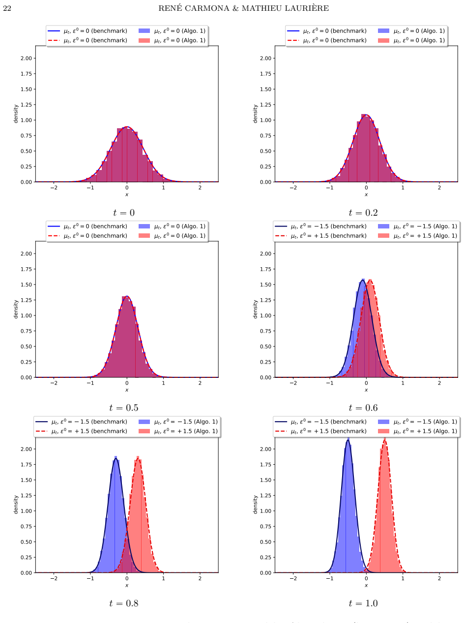
- [Section 5, numerical results] The text states that test cases 5 and 6 fall outside the scope of the theory, but test case 2 also falls outside, since its terminal cost g(x) = min(|x-xi_1|, |x-xi_2|) is non-smooth. Please make the limitation statement cover all three cases explicitly.
- [Remark 4 and Remark 11] After correcting the rate in Proposition 8 and Theorem 3, the discussion of the curse of dimensionality and of possible improvements should be updated to reflect the actual width exponent n_in^{-1/(6(d+1))} rather than the stated n_in^{-1/(3(d+1))}.
- [Appendix B] The proof of Proposition 7 quotes inequality (36) from [19, Theorem 6.17] and gives only a short derivation of the reduction to closed-loop controls. Since this step supplies the finite-population rate epsilon_1, please state the precise modification of the referenced theorem or provide the full argument, so that the main theorem is self-contained.
- [Throughout] There are minor typographical issues, including 'Apppendix A' in Remark 12 and the inconsistent spelling 'Bachmann-Landau'; these should be cleaned up in a revision.
Circularity Check
No significant circularity: the error decomposition is proven from external approximation theory and explicit estimates, not from fitted quantities or self-referential definitions.
full rationale
The paper's central bound (Theorem 3) is obtained by a three-step decomposition: finite-population approximation (Proposition 7), neural-network approximation (Proposition 8), and Euler time discretization (Proposition 15). None of these steps is defined in terms of the quantity being predicted: the proxy objective J_N(phi) is introduced as a new minimization problem (Problem 2), and the theorem bounds inf_alpha J(alpha) below by inf_phi J_N(phi) minus explicit rates. The neural-network rate eps_2 relies on the external approximation theorem of Mhaskar-Micchelli (Theorem 9), combined with a self-contained Lipschitz-stability estimate (Proposition 13), with no fitted constants. The Euler rate eps_3 is proved from a strong-error lemma (Lemma 14) and Ito estimates in Appendix D. Proposition 7 is imported from the authors' book [19, Theorem 6.17], a parameter-free published theorem whose stated assumptions do not include the present theorem; this is legitimate external evidence rather than a circular reduction. The paper's admitted limitations (Remark 5 leaving the stochastic-gradient/generalization error to future work; Section 5 noting that several test cases fall outside the theory) are scope limitations, not circularity. The apparent square-root gap in the displayed algebra of Proposition 8 is a proof-rate correctness issue, not a circularity, and does not change this verdict.
Assumptions & free parameters
assumptions (5)
- domain assumption Drift b is linear in x, μ, α; volatility σ is linear in x, μ (Assumption A1, Appendix A).
- domain assumption The forward-backward system (7) is uniquely solvable and admits a master field U, with decoupling field V jointly Lipschitz and twice differentiable in x with Lipschitz Bxx V (Assumptions B2, C2; Section 2.2).
- ad hoc to paper Conditions (C1)-(C3) on growth and smoothness of f and its derivatives, and of the Hamiltonian minimizer α̂ (Appendix A).
- standard math Mhaskar-Micchelli neural network approximation theorem and Schultz Jackson-type inequality for trigonometric polynomials (Theorem 9, Section 3.2).
- standard math Propagation of chaos bound from [19, Theorem 6.17] imported in Proposition 7.
Cite this review
Pith. "Pith review of Convergence Analysis of Machine Learning Algorithms for the Numerical Solution of Mean Field Control and Games: II -- The Finite Horizon Case." pith.science (2026). https://pith.science/paper/LTJQKDPB
@misc{pith2026190801613,
  author       = {Pith},
  title        = {Pith review of: Convergence Analysis of Machine Learning Algorithms for the Numerical Solution of Mean Field Control and Games: II -- The Finite Horizon Case},
  year         = {2026},
  howpublished = {\url{https://pith.science/paper/LTJQKDPB}},
  note         = {Machine review of arXiv:1908.01613}
}
read the original abstract
We propose two numerical methods for the optimal control of McKean-Vlasov dynamics in finite time horizon. Both methods are based on the introduction of a suitable loss function defined over the parameters of a neural network. This allows the use of machine learning tools, and efficient implementations of stochastic gradient descent in order to perform the optimization. In the first method, the loss function stems directly from the optimal control problem. The second method tackles a generic forward-backward stochastic differential equation system (FBSDE) of McKean-Vlasov type, and relies on suitable reformulation as a mean field control problem. To provide a guarantee on how our numerical schemes approximate the solution of the original mean field control problem, we introduce a new optimization problem, directly amenable to numerical computation, and for which we rigorously provide an error rate. Several numerical examples are provided. Both methods can easily be applied to certain problems with common noise, which is not the case with the existing technology. Furthermore, although the first approach is designed for mean field control problems, the second is more general and can also be applied to the FBSDE arising in the theory of mean field games.
Figures
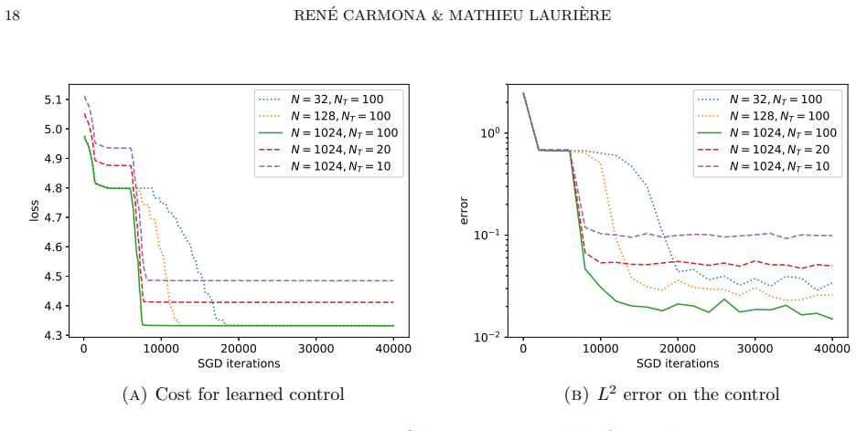
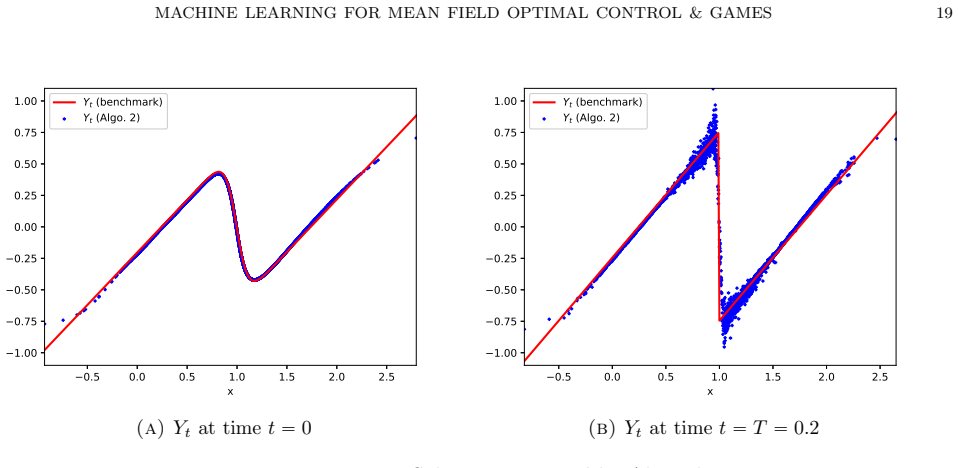
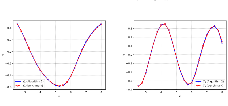
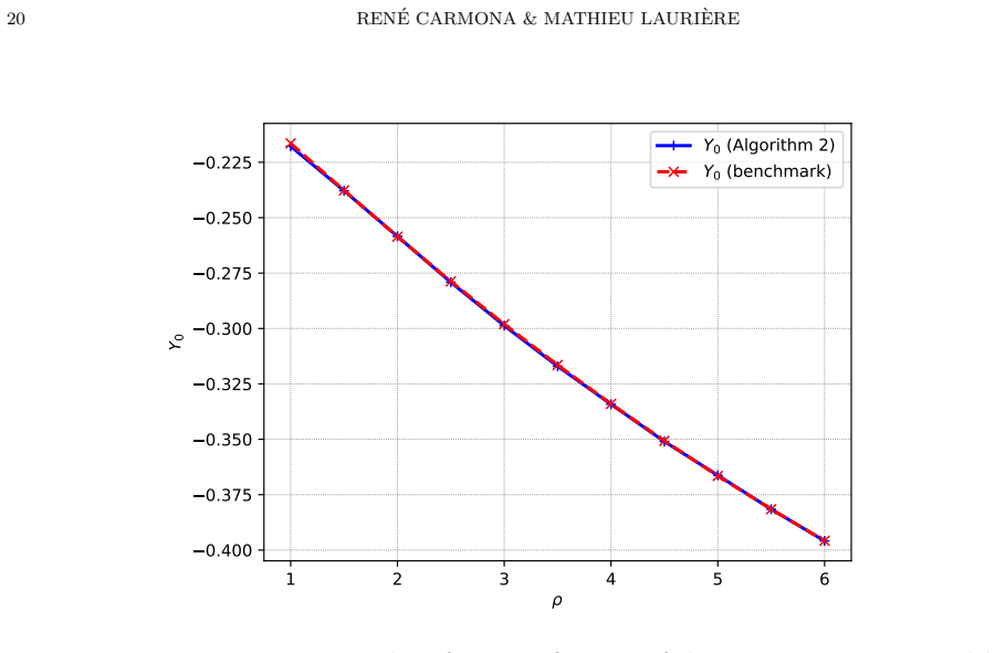
Figures from the paper (5 more)
Reference graph
Works this paper leans on
-
[1]
Mean field games: numerical methods for the planning problem
Yves Achdou, Fabio Camilli, and Italo Capuzzo-Dolcetta. Mean field games: numerical methods for the planning problem. SIAM J. Control Optim. , 50(1):77–109, 2012
work page 2012
-
[2]
Mean field games: numerical methods
Yves Achdou and Italo Capuzzo-Dolcetta. Mean field games: numerical methods. SIAM J. Numer. Anal. , 48(3):1136– 1162, 2010
work page 2010
-
[3]
Mean field games for modeling crowd motion
Yves Achdou and Jean-Michel Lasry. Mean field games for modeling crowd motion. In Boris N. Chetverushkin, William Fitzgibbon, Yuri A. Kuznetsov, Pekka Neittaanm¨ aki, Jacques Periaux, and Olivier Pironneau, editors,Contributions to Partial Differential Equations and Applications , chapter 4, pages 17–42. Springer International Publishing, 2019
work page 2019
-
[4]
On the system of partial differential equations arising in mean field type control
Yves Achdou and Mathieu Lauri` ere. On the system of partial differential equations arising in mean field type control. Discrete Contin. Dyn. Syst. , 35(9):3879–3900, 2015
work page 2015
-
[5]
Mean Field Type Control with Congestion (II): An augmented Lagrangian method
Yves Achdou and Mathieu Lauri` ere. Mean Field Type Control with Congestion (II): An augmented Lagrangian method. Appl. Math. Optim. , 74(3):535–578, 2016
work page 2016
-
[6]
Two numerical approaches to stationary mean-field games
Noha Almulla, Rita Ferreira, and Diogo Gomes. Two numerical approaches to stationary mean-field games. Dyn. Games Appl., 7(4):657–682, 2017
work page 2017
-
[7]
Graves, Houzhi Li, Jean-Fran¸ cois Chassagneux, Fran¸ cois Delarue, and Ren´ e Carmona
Andrea Angiuli, Christy V. Graves, Houzhi Li, Jean-Fran¸ cois Chassagneux, Fran¸ cois Delarue, and Ren´ e Carmona. CEMRACS 2017: numerical probabilistic approach to MFG. In CEMRACS 2017—numerical methods for stochastic models: control, uncertainty quantification, mean-field , volume 65 of ESAIM Proc. Surveys, pages 84–113. EDP Sci., Les Ulis, 2019
work page 2017
-
[8]
A class of finite-dimensional numerically solvable McKean-Vlasov control problems
Alessandro Balata, Cˆ ome Hur´ e, Mathieu Lauri` ere, Huyˆ en Pham, and Isaque Pimentel. A class of finite-dimensional numerically solvable McKean-Vlasov control problems. ESAIM: Proceedings and Surveys, 65:114–144, 2019
work page 2019
Show all 38 references
-
[9]
Mean field games and mean field type control theory
Alain Bensoussan, Jens Frehse, and Sheung Chi Phillip Yam. Mean field games and mean field type control theory . Springer Briefs in Mathematics. Springer, New York, 2013
2013
-
[10]
A stochastic particle method for the McKean-Vlasov and the Burgers equation
Mireille Bossy and Denis Talay. A stochastic particle method for the McKean-Vlasov and the Burgers equation. Math. Comp., 66(217):157–192, 1997
1997
-
[11]
Curtis, and Jorge Nocedal
L´ eon Bottou, Frank E. Curtis, and Jorge Nocedal. Optimization methods for large-scale machine learning.SIAM Rev., 60(2):223–311, 2018. MACHINE LEARNING FOR MEAN FIELD OPTIMAL CONTROL & GAMES 43
2018
-
[12]
Brice˜ no Arias, Dante Kalise, Ziad Kobeissi, Mathieu Lauri` ere, ´Alvaro Mateos Gonz´ alez, and Francisco J
Luis M. Brice˜ no Arias, Dante Kalise, Ziad Kobeissi, Mathieu Lauri` ere, ´Alvaro Mateos Gonz´ alez, and Francisco J. Silva. On the implementation of a primal-dual algorithm for second order time-dependent mean field games with local couplings. ESAIM: ProcS, 65:330–348, 2019
2019
-
[13]
Brice˜ no Arias, Dante Kalise, and Francisco J
Luis M. Brice˜ no Arias, Dante Kalise, and Francisco J. Silva. Proximal methods for stationary mean field games with local couplings. SIAM J. Control Optim. , 56(2):801–836, 2018
2018
-
[14]
An ergodic problem for mean field games: qualitative properties and numerical simulations
Simone Cacace, Fabio Camilli, Annalisa Cesaroni, and Claudio Marchi. An ergodic problem for mean field games: qualitative properties and numerical simulations. Minimax Theory Appl. , 3(2):211–226, 2018
2018
-
[15]
Cardaliaguet, F
P. Cardaliaguet, F. Delarue, J.M. Lasry, and P.L. Lions. The Master Equation and the Convergence Problem in Mean Field Games. Annals of Mathematics Studies. Princeton University Press, 2019
2019
-
[16]
Notes on mean field games
Pierre Cardaliaguet. Notes on mean field games. 2013
2013
-
[17]
Elisabetta Carlini and Francisco J. Silva. A fully discrete semi-Lagrangian scheme for a first order mean field game problem. SIAM J. Numer. Anal. , 52(1):45–67, 2014
2014
-
[18]
I , volume 83 of Probability Theory and Stochastic Modelling
Ren´ e Carmona and Fran¸ cois Delarue.Probabilistic theory of mean field games with applications. I , volume 83 of Probability Theory and Stochastic Modelling . Springer, Cham, 2018. Mean field FBSDEs, control, and games
2018
-
[19]
II , volume 84 of Probability Theory and Stochastic Modelling
Ren´ e Carmona and Fran¸ cois Delarue.Probabilistic theory of mean field games with applications. II , volume 84 of Probability Theory and Stochastic Modelling. Springer, Cham, 2018. Mean field games with common noise and master equations
2018
-
[20]
Mean field games and systemic risk
Ren´ e Carmona, Jean-Pierre Fouque, and Li-Hsien Sun. Mean field games and systemic risk. Commun. Math. Sci. , 13(4):911–933, 2015
2015
-
[21]
Machine learning for the optimal control of MKV dynamics and mean field games I: The ergodic case
Ren´ e Carmona and Mathieu Lauri` ere. Machine learning for the optimal control of MKV dynamics and mean field games I: The ergodic case. arXiv preprint, arXiv:1907.05980, 2019
1907 arXiv
-
[22]
A probabilistic approach to classical solutions of the master equation for large population equilibria
Jean-Fran¸ cois Chassagneux, Dan Crisan, and Fran¸ cois Delarue. A probabilistic approach to classical solutions of the master equation for large population equilibria. arXiv:1411.3009, 2014
2014 arXiv
-
[23]
Numerical method for FBSDEs of McKean-Vlasov type
Jean-Fran¸ cois Chassagneux, Dan Crisan, and Fran¸ cois Delarue. Numerical method for FBSDEs of McKean-Vlasov type. Ann. Appl. Probab., 29(3):1640–1684, 2019
2019
-
[24]
Dynamic programming approach to principal-agent problems
Jakˇ sa Cvitani´ c, Dylan Possama¨ ı, and Nizar Touzi. Dynamic programming approach to principal-agent problems. Finance Stoch., 22(1):1–37, 2018
2018
-
[25]
Springer Finance
Jakˇ sa Cvitani´ c and Jianfeng Zhang.Contract theory in continuous-time models . Springer Finance. Springer, Heidel- berg, 2013
2013
-
[26]
Deep learning-based numerical methods for high-dimensional parabolic partial differential equations and backward stochastic differential equations.Commun
Weinan E, Jiequn Han, and Arnulf Jentzen. Deep learning-based numerical methods for high-dimensional parabolic partial differential equations and backward stochastic differential equations.Commun. Math. Stat., 5(4):349–380, 2017
2017
-
[27]
Deep learning methods for mean field control problems with delay
Jean-Pierre Fouque and Zhaoyu Zhang. Deep learning methods for mean field control problems with delay. arXiv:1905.00358, 2019
1905 arXiv
-
[28]
Sensitivity analysis using Itˆ o-Malliavin calculus and martingales, and application to stochastic optimal control
Emmanuel Gobet and R´ emi Munos. Sensitivity analysis using Itˆ o-Malliavin calculus and martingales, and application to stochastic optimal control. SIAM J. Control Optim. , 43(5):1676–1713, 2005
2005
-
[29]
Deep learning approximation for stochastic control problems.Deep Reinforcement Learning Workshop, NIPS, arXiv preprint arXiv:1611.07422 , 2016
Jiequn Han and Weinan E. Deep learning approximation for stochastic control problems.Deep Reinforcement Learning Workshop, NIPS, arXiv preprint arXiv:1611.07422 , 2016
2016 arXiv
-
[30]
Convergence of the deep bsde method for coupled fbsdes
Jiequn Han and Jihao Long. Convergence of the deep bsde method for coupled fbsdes. Probability, Uncertainty and Quantitative Risk, 5(1):1–33, 2020
2020
-
[31]
Relationship between backward stochastic differential equations and stochastic controls: a linear-quadratic approach
Michael Kohlmann and Xun Yu Zhou. Relationship between backward stochastic differential equations and stochastic controls: a linear-quadratic approach. SIAM J. Control Optim. , 38(5):1392–1407, 2000
2000
-
[32]
Mean field games
Jean-Michel Lasry and Pierre-Louis Lions. Mean field games. Jpn. J. Math. , 2(1):229–260, 2007
2007
-
[33]
Dynamic programming for mean-field type control.J
Mathieu Lauri` ere and Olivier Pironneau. Dynamic programming for mean-field type control.J. Optim. Theory Appl. , 169(3):902–924, 2016
2016
-
[34]
Mhaskar and Charles A
Hrushikesh N. Mhaskar and Charles A. Micchelli. Degree of approximation by neural and translation networks with a single hidden layer. Advances in Applied Mathematics , 16:151–183, 1995
1995
-
[35]
Numerical methods for mean-field type optimal control problems
Laurent Pfeiffer. Numerical methods for mean-field type optimal control problems. Pure Appl. Funct. Anal., 1(4):629– 655, 2016
2016
-
[36]
Malham´ e, and J´ erˆ ome Le Ny
Rabih Salhab, Roland P. Malham´ e, and J´ erˆ ome Le Ny. A dynamic game model of collective choice in multi-agent systems. In 2015 IEEE 54th Annual Conference on Decision and Control (CDC) , pages 4444–4449, Osaka, Japon, December 2015
2015
-
[37]
Martin H. Schultz. L8-multivariate approximation theory. SIAM J. Numer. Anal. , 6:184–209, 1969. 44 REN ´E CARMONA & MATHIEU LAURI `ERE
1969
-
[38]
Topics in propagation of chaos
Alain-Sol Sznitman. Topics in propagation of chaos. In ´Ecole d’ ´Et´ e de Probabilit´ es de Saint-Flour XIX—1989, volume 1464 of Lecture Notes in Math. , pages 165–251. Springer, Berlin, 1991
1989
Reviewed August 14, 2026 · model on record in the stance chip above.
Discussion (0). Continue with ORCID to comment.