REVIEW 4 major objections 4 minor 27 references
Projecting the nominal drift onto the measurement-consistent subspace yields a geometry-consistent particle proposal that provably preserves the Bayesian posterior while reducing importance-weight variance, with large accuracy and diversity
Reviewed by Pith at T0; open to challenge. T0 means a machine referee read the full paper against a public rubric. the ladder, T0–T4 →
T0 review · deepseek-v4-flash
2026-08-01 17:02 UTC pith:M4A5DIXC
load-bearing objection The geometric projection idea is worth a look, but the weight update in Algorithm 1 is not the importance weight for its own proposal, so the posterior-preservation theorems don't cover the implemented filter. the 4 major comments →
Geometry-Consistent Bayesian Filtering under Structural Model Uncertainty: A Geometric Projection Particle Filter
The pith
A machine-rendered reading of the paper's core claim, the machinery that carries it, and where it could break.
Core claim
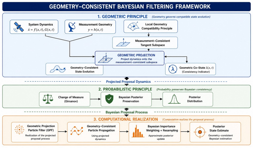
The paper's central claim is that enforcing local compatibility between state propagation and measurement geometry — via the constraint H_t dx_t + ∂_t h dt = dy_t - dW_t — produces a projected stochastic dynamics dx = P_⊥ f dt + P_∥(dy - ∂_t h dt - dW_t), where P_∥ = H^T(HH^T)^†H and P_⊥ = I - P_∥. The paper proves this projected proposal has a unique strong solution, preserves the Bayesian posterior through the Kallianpur–Striebel representation, and gives a self-normalized particle approximation converging at the standard O(N^{-1/2}) rate. It further establishes an error decomposition showing that structural model mismatch only propagates when it lies orthogonal to the measurement-consiste
What carries the argument
The central object is the orthogonal projection operator P_∥ = H^T (H H^T)^† H, where H is the measurement Jacobian, and its complement P_⊥ = I - P_∥. These project the nominal drift onto (respectively away from) the subspace that instantaneously affects the measurement. The projected proposal dx = P_⊥ f dt + P_∥(dy - ∂_t h dt - dW_t) and the geometric co-state λ = (HH^T)^†(dy - H f dt - ∂_t h dt - dW_t) carry the argument: the co-state is an intrinsic estimator-integrity indicator, and the change of measure via the likelihood process L_t = exp(∫ η^T dy - ½∫‖η‖² dt) is what keeps the posterior intact.
Load-bearing premise
The load-bearing premise is that the discrete weight update log w += η^T Δy - ½‖η‖² Δt is exactly the correct importance weight for the projected proposal in Algorithm 1 — but the algorithm never evaluates the proposal density q, so the posterior-preservation theorem may not transfer from continuous time to the implemented discretization.
What would settle it
Run GPF on a linear-Gaussian state-space model where the exact posterior is known from the Kalman filter; if the GPF estimate's mean and covariance deviate beyond Monte Carlo error, the claimed posterior preservation fails. More directly, compute the actual proposal density q in Algorithm 1 and compare the algorithm's log-weight increment to log[p(y_{k+1}|x_{k+1}) p(x_{k+1}|x_k) / q(x_{k+1}|x_k, y_{k+1})]; any mismatch would falsify the discrete-time claim.
If this is right
- If posterior preservation holds, existing bootstrap particle filter implementations can be upgraded by changing only the proposal step, leaving likelihood weighting and resampling untouched.
- The error bound implies that model mismatch aligned with the measurement subspace is automatically corrected by the projection; only the orthogonal component contributes to estimation error.
- The geometric co-state provides a computable, online indicator of model mismatch, enabling real-time monitoring of estimator integrity without altering the Bayesian weights.
- The O(N^{-1/2}) Monte Carlo convergence rate is preserved, so the geometric projection adds robustness without sacrificing the standard SMC convergence guarantees.
- Under partial observability, the regularized pseudoinverse keeps the projection well-defined, so the framework extends to rank-deficient measurement configurations.
Where Pith is reading between the lines
- Beyond the paper, the same projection idea could be applied to ensemble Kalman filters by projecting forecast ensemble perturbations onto the measurement-consistent subspace, potentially reducing the need for covariance inflation under model error.
- The robustness bound suggests a counterintuitive design rule: when structural mismatch is known to lie in the measurement subspace, the projection should have little effect; its value is specifically for mismatch orthogonal to what is measured — a distinction that could guide where model refinement effort pays off.
- If the continuous-time proposal is taken literally, the discrete algorithm's omission of the dW term in the projection may be more than a numerical convenience; one testable extension is to include that noise-induced drift and check whether posterior preservation still holds in finite-sample benchmarks.
- The geometric co-state could be repurposed as a fault-detection statistic: since it is zero-mean under correct model specification, a running test on its magnitude would flag the onset of structural model change in real time.
Editorial analysis
A structured set of objections, weighed in public.
Referee Report
Summary. The paper proposes a 'geometry-consistent' proposal for continuous-time nonlinear filtering. The nominal drift is projected onto the range of the measurement Jacobian, producing a proposal SDE (Eq. 12) and a 'geometric co-state' λ_t that is claimed to quantify dynamics–measurement mismatch. The main theoretical claims are: well-posedness of the projected dynamics (Thm 3.13), zero-mean co-state under correct specification (Thm 3.7), posterior preservation through a Girsanov/Kallianpur–Striebel change of measure (Thm 4.2), convergence of an associated particle approximation (Thm 4.3), and an error decomposition under model mismatch (Prop. 4.4, Thm 4.5). The algorithmic realization is the Geometric Projection Particle Filter (GPF), Algorithm 1, which is tested on a lunar descent problem and reported to achieve higher ESS and lower RMSE than bootstrap particle, EKF, UKF, and EnKF baselines.
Significance. If the central posterior-preservation claim were correct, the paper would offer a principled way to build measurement-dependent proposals for particle filtering under model uncertainty, and the geometric co-state would be a useful diagnostic. The experimental framing (two observability cases, Monte Carlo statistics, ESS analysis, co-state/degeneracy plots) is a strength, as is the explicit pseudocode. However, the load-bearing Bayesian argument is not carried through to the implemented algorithm: the weight recursion in Algorithm 1 is not the importance-weight recursion derived in Eq. (26), and the change-of-measure theorem does not apply to the process actually simulated. The empirical improvements may be real for a heuristic nudged filter, but they do not validate the paper's claimed Bayesian foundation. Because the central theoretical claims fail for the delivered algorithm, the paper in its present form cannot be accepted.
major comments (4)
- [§5.2 / Algorithm 1] Algorithm 1's weight update is not the importance-weight recursion of Eq. (26). Line 9 propagates particles with a proposal q(x_{k+1}|x_k,y_{k+1}) that uses Δy_k; line 10 increments log w by η^T Δy − ½∥η∥² Δt. Eq. (26) requires the factor p(y_{k+1}|x_{k+1}) p(x_{k+1}|x_k) / q(x_{k+1}|x_k,y_{k+1}), and none of these densities is evaluated anywhere in the algorithm. In the small-diffusion limit the proposal is a point mass conditionally on the measurement, and no scalar weight increment of the stated form can repair the missing proposal-density ratio. The implemented GPF is therefore a nudged/projection filter, not a self-normalized importance sampler, and Theorems 4.2 and 4.3 do not apply to it.
- [§3.3, Theorem 3.7, Eq. (12)] Under the stated model (1)–(2), the observation differential is d y_t = d h(x_t,t) + dW_t, so under correct model specification the reference innovation is dν_t = H_t G_t dB_t + dW_t (plus second-order Itô terms), not dW_t as claimed in §3.3. Consequently Theorem 3.7's conclusion E[λ_t|F^y_t]=0 is not established. Relatedly, the projected SDE (12) contains an explicit −dW_t term and no G_t dB_t diffusion term, so the continuous-time proposal is not consistent with the discrete Euler step in Algorithm 1, which adds G(x,t)√Δt ξ but does not subtract a measurement-noise increment. The connection between the continuous-time construction and the discrete algorithm is left unjustified.
- [§4.1, Eq. (17), Theorem 4.2] The change-of-measure argument does not prove posterior preservation. Eq. (17) chooses η as the observation drift in the Girsanov density, but the actual observation model (1)–(2) has a noise component H G dB_t + dW_t and a drift containing H f + ∂_t h (again with Itô correction); Eq. (17) is not the Radon–Nikodym derivative for that observation model. Moreover, the proposal process (12) is adapted to F^y_t, so substituting the proposal into the Kallianpur–Striebel formula (20) does not yield the posterior of the original signal. The theorem asserts the equality EP[u(x_t)|F^y_t] = EQ[u(x_t)L_t]/EQ[L_t] without identifying which x_t (original signal or proposal) enters and without deriving the density relationship that would make the equality true.
- [§4.3, Proposition 4.4 / Theorem 4.5] The error decomposition is not derived rigorously. The proposal process (12) is driven by innovation/λ terms in addition to the projected drift, so the evolution of e(t)=x_true(t)−x(t) cannot be written simply as ˙e=(I−P∥)Δf+λ without additional terms; λ in Eq. (15) is itself a function of the innovation and is not an independent residual process. The bound (23) is then an immediate triangle inequality from an assumed ODE that is never obtained from the SDEs (1) and (12). As written, Proposition 4.4 and Theorem 4.5 provide an interpretation, not a proof, of robustness.
minor comments (4)
- [§3.2, Eq. (4)] The statement that 'higher-order Itô terms are neglected' is an approximation, but Theorem 4.2 claims exact posterior preservation. The paper should either quantify the discretization/Itô error or state the claims as approximate.
- [Algorithm 1, lines 5–9] It is unclear whether H^{(i)}_{t_k} is evaluated at the predicted state x^{i,-}_{t_k} or at the filtered/projected state x^{i}_{t_k}; line 5 says only 'compute Jacobian.' This affects the projection and should be stated explicitly.
- [§7.1 / Remark 3.6] The Tikhonov parameter ε, the resampling threshold τ (N/2 in the text, τN in Algorithm 1), and ϵ_dyn are all free parameters, but ε and τ are not reported in the experiments. Values should be given for reproducibility.
- [§4.2, Eq. (22)] The weights are defined as proportional to the unbounded process L_t^{(i)}, yet Theorem 4.3 assumes 'finite second moments and non-degenerate importance weights' without checking them for L_t. This is nontrivial for the continuous-time likelihood and should be addressed.
Circularity Check
No significant circularity: the main issue is a theory/algorithm mismatch, not a prediction that reduces to its inputs.
full rationale
Walking the derivation chain, I find no step in which a claimed prediction or first-principles result is equivalent to its inputs by construction. The continuous-time projected dynamics (12) are obtained by algebraically eliminating the co-state λ from the compatibility condition, and the well-posedness result is a standard Lipschitz/linear-growth SDE argument. Theorem 4.2 is an application of the external Kallianpur–Striebel/Girsanov identity; the proof does restate the KS representation, but the KS formula is an independent classical result rather than a self-citation or an assumption smuggled in through the paper's own definitions. There are no load-bearing self-citations, no fitted parameters later renamed as predictions, and no uniqueness/ansatz imported from the authors' prior work. The genuine weakness is that Algorithm 1's weight update (line 10) does not evaluate the proposal density q appearing in the declared importance-weight recursion (26), so the implemented filter is not obviously the importance sampler analyzed in Theorems 4.2–4.3. That is a correctness/convergence gap, not a circular dependency: the paper does not derive the claimed posterior preservation from the very quantity it is trying to predict. Likewise, the reported ESS/RMSE improvements are structurally plausible consequences of a proposal that conditions particle propagation on the current measurement, but an improved proposal by design is the paper's contribution, not a circular prediction of its own output. I therefore find no significant circularity and score 0.
Axiom & Free-Parameter Ledger
free parameters (3)
- Tikhonov regularization epsilon =
not specified
- Resampling threshold tau =
not specified in Algorithm 1; experiments use N/2
- Model mismatch magnitude eps_dyn =
0.09 (9%)
axioms (4)
- standard math Assumptions 3.9–3.11: f, G, h are C^1/locally Lipschitz with linear growth; H progressively measurable locally bounded; (H H^T)^† locally Lipschitz bounded.
- domain assumption Assumption 4.1 (Novikov condition on eta) holds.
- domain assumption Observation model (2): y_t = h(x_t,t) + W_t with W a standard Wiener process, used as the basis for the change-of-measure.
- ad hoc to paper Implicit assumption behind Algorithm 1: the importance weight can be updated by the observation likelihood alone, without the proposal-density ratio p(x_{k+1}|x_k)/q(x_{k+1}|x_k,y_{k+1}).
invented entities (1)
-
geometric co-state lambda_t
no independent evidence
read the original abstract
Nonlinear state estimation under structural model uncertainty remains a fundamental challenge in autonomous Guidance, Navigation, and Control (GNC) systems. Conventional Bayesian filtering separates state propagation from measurement correction, allowing model mismatch to accumulate during propagation, resulting in proposal--likelihood inconsistency, particle degeneracy, and degraded estimation accuracy. Existing approaches primarily improve proposal distributions or weighting strategies without explicitly incorporating measurement geometry into state propagation. This paper introduces a geometry-consistent Bayesian filtering framework that incorporates measurement geometry directly into the propagation process. The nominal drift is projected onto the measurement-consistent subspace, yielding a geometry-consistent proposal while preserving the Bayesian posterior through a rigorous change-of-measure formulation. A Geometric Projection Particle Filter (GPF) is developed together with a geometric co-state that quantifies instantaneous dynamics--measurement inconsistency. Theoretical analysis establishes existence and uniqueness of the projected dynamics, posterior preservation, standard Monte Carlo convergence of the particle approximation, and robustness under structural model uncertainty. The framework is validated using lunar descent navigation under partial observability and persistent model uncertainty. Compared with the bootstrap particle filter and conventional Gaussian filtering methods, GPF consistently achieves higher effective sample size and lower estimation error. These results demonstrate that geometry-consistent propagation provides a principled, computationally efficient, and theoretically grounded framework for robust nonlinear Bayesian filtering.
Figures


Reference graph
Works this paper leans on
-
[1]
R. E. Kalman, A new approach to linear filtering and prediction problems, Journal of Basic Engineering 82 (1) (1960) 35–45
1960
-
[2]
R. E. Kalman, R. S. Bucy, New results in linear filtering and prediction theory, Journal of Basic Engineering 83 (1) (1961) 95–108
1961
-
[3]
P. S. Maybeck, Stochastic Models, Estimation, and Con- trol, Academic Press, 1979
1979
-
[4]
J. L. Crassidis, J. L. Junkins, Optimal Estimation of Dy- namic Systems, CRC Press, 2012
2012
-
[5]
Doucet, N
A. Doucet, N. de Freitas, N. Gordon, Sequential Monte Carlo Methods in Practice, Springer, 2001
2001
-
[6]
M. S. e. a. Arulampalam, A tutorial on particle filters, IEEE Transactions on Signal Processing 50 (2) (2002) 174–188. 12
2002
-
[7]
A. Kong, J. S. Liu, W. H. Wong, Sequential imputations and bayesian missing data problems, Journal of the Amer- ican Statistical Association 89 (425) (1994) 278–288
1994
-
[8]
R. Douc, O. Capp’e, Comparison of resampling schemes for particle filtering, Proceedings of ISPA (2005)
2005
-
[9]
Snyder, T
C. Snyder, T. Bengtsson, P. Bickel, J. Anderson, Obstacles to high-dimensional particle filtering, Monthly Weather Review 136 (12) (2008) 4629–4640
2008
-
[10]
M. K. Pitt, N. Shephard, Filtering via simulation: Aux- iliary particle filters, Journal of the American Statistical Association 94 (446) (1999) 590–599
1999
-
[11]
Doucet, S
A. Doucet, S. Godsill, C. Andrieu, On sequential monte carlo sampling methods for bayesian filtering, Statistics and Computing 10 (2000) 197–208
2000
-
[12]
A. J. e. a. Chorin, Implicit particle filters, Communica- tions in Applied Mathematics (2010)
2010
-
[13]
A. J. Chorin, X. Tu, Implicit sampling, PNAS (2015)
2015
-
[14]
F. Daum, J. Huang, Particle flow for nonlinear filters, Pro- ceedings of SPIE (2011)
2011
-
[15]
Reich, A nonparametric ensemble transform method for bayesian inference, SIAM Journal on Scientific Com- puting 35 (4) (2013) A2013–A2024
S. Reich, A nonparametric ensemble transform method for bayesian inference, SIAM Journal on Scientific Com- puting 35 (4) (2013) A2013–A2024
2013
-
[16]
Bunch, S
P. Bunch, S. Godsill, Particle filters for continuous time stochastic processes using forward transport, IEEE Trans- actions on Signal Processing 64 (8) (2016) 1937–1950
2016
-
[17]
P. J. e. a. van Leeuwen, Particle filters for high- dimensional systems, Quarterly Journal of the Royal Me- teorological Society (2019)
2019
-
[18]
P. G. Mehta, S. P. Meyn, Feedback particle filter, IEEE Transactions on Automatic Control 57 (10) (2012) 2665– 2671
2012
-
[19]
Song, et al., Score-based generative modeling through stochastic differential equations, ICLR (2021)
Y . Song, et al., Score-based generative modeling through stochastic differential equations, ICLR (2021)
2021
-
[20]
Levy, Robust bayesian filtering under model uncer- tainty, IEEE TAC (2017)
B. Levy, Robust bayesian filtering under model uncer- tainty, IEEE TAC (2017)
2017
-
[21]
Procope-Mamert, N
S. Procope-Mamert, N. Chopin, M. Delattre, A forward- only scheme for online learning of proposal distributions in particle filters, Journal of Computational and Graphical Statistics (2026)
2026
-
[22]
Zhang, et al., State estimation with model uncertainty using structure variational bayesian and transfer learning, IEEE/CAA Journal of Automatica Sinica 12 (3) (2025)
L. Zhang, et al., State estimation with model uncertainty using structure variational bayesian and transfer learning, IEEE/CAA Journal of Automatica Sinica 12 (3) (2025)
2025
-
[23]
J. A. Rebollo, F. Gavilan, R. Vazquez, A symmetry- based unscented particle filter for rapid state esti- mation for sal guided vehicles, IEEE Transactions on Aerospace and Electronic Systems (2024) 1– 13doi:10.1109/TAES.2024.3475995
arXiv 2024
-
[24]
G. Fang, Y . Zhang, P. Zhang, Y . Lu, P. Huang, Full state estimation for triangular tethered satellite forma- tions: Filter design, observability analysis, and per- formance evaluation, IEEE Transactions on Aerospace and Electronic Systems 60 (6) (2024) 7277–7291. doi:10.1109/TAES.2024.3415573
arXiv 2024
- [25]
-
[26]
Xiong, An Introduction to Stochastic Filtering Theory, Oxford University Press, 2008
J. Xiong, An Introduction to Stochastic Filtering Theory, Oxford University Press, 2008
2008
-
[27]
Del Moral, Feynman-Kac Formulae: Genealogical and Interacting Particle Systems with Applications, Springer, 2004
P. Del Moral, Feynman-Kac Formulae: Genealogical and Interacting Particle Systems with Applications, Springer, 2004. 13
2004
discussion (0)
Sign in with ORCID, Apple, or X to comment. Anyone can read and Pith papers without signing in.