REVIEW 3 major objections 5 minor 129 references
Frontier coding agents fail systematically on scientific imaging pipelines in ways general coding benchmarks never show.
Reviewed by Pith at T0; open to challenge. T0 means a machine referee read the full paper against a public rubric. the ladder, T0–T4 →
T0 review · grok-4.5
2026-07-14 09:14 UTC pith:M6KD4ZJY
load-bearing objection Solid, carefully built inverse-problem coding benchmark; the multi-track evidence for convention and solver failures is real, with residual risk only on end-to-end image metrics. the 3 major comments →
Imaging-101: Benchmarking LLM Coding Agents on Scientific Computational Imaging
The pith
A machine-rendered reading of the paper's core claim, the machinery that carries it, and where it could break.
Core claim
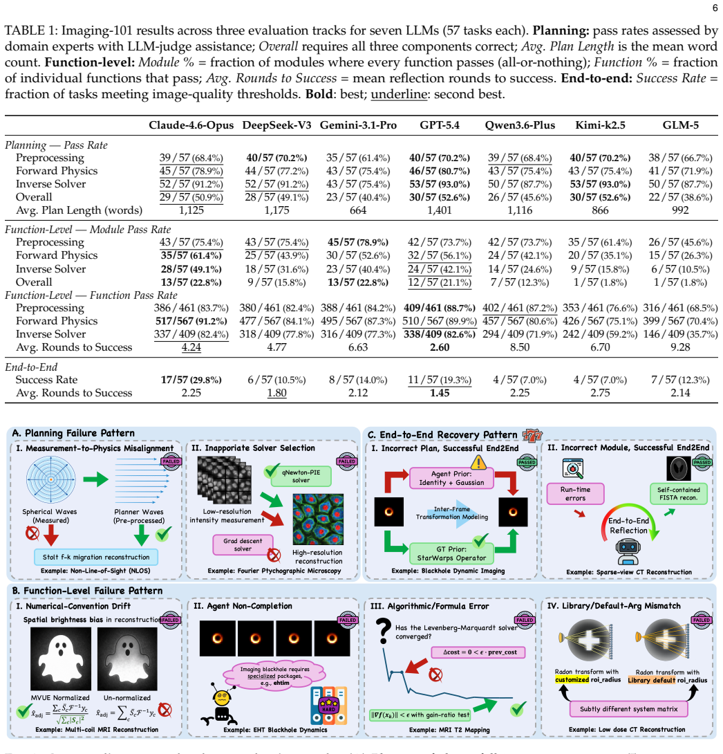
On 57 paper-grounded computational imaging tasks, frontier LLM coding agents systematically fail at algorithm selection, physical convention handling, and pipeline integration—failure modes that general coding and science-QA benchmarks do not expose. Controlled end-to-end success peaks at 29.8 percent, while simultaneous pass of all three scientific modules ranges only from 1.8 to 22.8 percent across models.
What carries the argument
Imaging-101: every task is canonicalized into a standardized four-stage pipeline (preprocessing, forward physics modeling, inverse solver, visualization) and graded on three tracks—planning, function-level numerical unit tests, and end-to-end reconstruction against calibrated image-quality thresholds.
Load-bearing premise
The evaluation treats expert plan judgments plus calibrated image-quality cutoffs as enough proof of scientific correctness, even though a physically wrong pipeline can still look plausible and pass those image metrics.
What would settle it
Rerun the same 57-task suite under the same multi-agent harness and reflection budget with a stronger model or skill library; if end-to-end rates rise high while function-level fixtures and expert plan rubrics also pass on convention-sensitive tasks (for example multi-coil MRI normalization and NLOS intensity-to-amplitude conversion), the claim of systematic scientific-reasoning gaps would not hold.
If this is right
- Reliable imaging copilots will need reusable, verified skill modules that encode tacit conventions such as normalizations, unit conversions, and modality-specific solvers.
- Getting the algorithmic plan right has a larger effect on final reconstruction success than perfecting every individual function in isolation.
- Image-quality scores alone cannot certify physical correctness, so multi-track evaluation (plan, unit tests, end-to-end) is required to catch convention drift.
- Richer execution environments (shell, packages, free debugging) can substantially raise pass rates relative to sandboxed multi-agent setups.
- New tasks can be added by the same expert-in-the-loop four-stage canonicalization, enabling community growth of the benchmark.
Where Pith is reading between the lines
- The same defaulting to statistically dominant conventions likely appears in other inverse-problem fields where minority physical conventions are underrepresented in training data.
- Injecting verified physics modules at code-writing time, not only at test time, may directly attack the dominant convention-drift failure class.
- The large gap between planning pass rates and end-to-end success points to long-horizon integration as a distinct research target from single-function coding skill.
Editorial analysis
A structured set of objections, weighed in public.
Referee Report
Summary. The manuscript introduces Imaging-101, a benchmark of 57 expert-verified computational imaging tasks spanning six scientific domains. Each task is grounded in a peer-reviewed paper and open-source reference, then canonicalized into a four-stage pipeline (preprocessing, forward physics, inverse solver, visualization). Three tracks—planning (expert binary judgments with LLM-judge assistance), function-level unit tests with reflection, and end-to-end reconstruction under a shared multi-agent harness—evaluate seven frontier LLMs. Results show low overall planning pass rates (~39–53%), very low all-module function-level success (1.8–22.8%), and end-to-end success at most 29.8% (Claude-4.6-Opus; 56.1% for black-box Claude Code). Dominant failures are scientific rather than purely syntactic: measurement-to-model misalignment, inappropriate solver selection, numerical-convention drift, and pipeline integration. The authors argue these gaps exceed those of general coding benchmarks and motivate skill-augmented, domain-specialized agents.
Significance. If the multi-track evidence holds, Imaging-101 is a substantial contribution: it fills a clear gap between clean-interface scientific coding benchmarks and the inverse-problem nature of computational imaging, with unusually careful expert-in-the-loop construction (12 domain experts, dual verification, paper-grounded references, calibrated fixtures). The case studies (NLOS intensity-to-amplitude conversion, MVUE coil normalization, FPM solver substitution) and the cross-tabulation of planning vs. function-level vs. end-to-end (Table 2) give concrete, falsifiable characterizations of failure modes that general coding suites rarely isolate. Releasing standardized tasks, plans, fixtures, and tutorials further supports community extension. The residual risk that NCC/NRMSE can accept physically wrong but visually plausible pipelines is acknowledged by the authors and partially bounded by the planning and function-level tracks; it does not erase the empirical value of the suite.
major comments (3)
- §2.3 Stage 3 and §3.3: End-to-end pass criteria (0.9× reference NCC, 1.1× reference NRMSE) can accept physically incorrect pipelines, as the authors themselves show for convention drift and the StarWarps black-hole case. Intermediate physics checks are deliberately omitted end-to-end. For the central claim that failures are scientific (not just coding), the paper should either (i) report, for a subset of end-to-end passes, whether planning and/or function-level physics checks also pass, or (ii) add a short multi-instance / alternative-metric analysis (promised in Appendix C.4) so that a single favorable instance cannot mask a missing prior. Without this, the softest joint of the multi-track argument remains under-quantified.
- §2.4.4–2.4.5 and Table 1: Controlled end-to-end results use a single self-developed multi-agent harness with fixed reflection budgets; Claude Code is reported separately at 56.1%. The claim that performance differences primarily reflect model capability (rather than harness idiosyncrasy) is plausible but load-bearing. A brief sensitivity check—e.g., one alternative agent scaffold or budget on a stratified subset—would strengthen attribution. If infeasible, state more explicitly that reported numbers are joint model–harness capability, not pure model ability.
- §4.2 and Appendix C.3: “Probabilistic mode collapse” is introduced as the analogue of the knowing–doing gap, supported mainly by 50 repeats of Claude-4.6-Opus on mri_l1_wavelet (47/50 convention-drift failures). That is useful but narrow. Either broaden the repeatability evidence to a few more convention-sensitive tasks/models, or temper the generality of the term so it is not read as a fully established mechanism across the suite.
minor comments (5)
- Abstract and §1: minor grammar (“visualization) Three evaluation tracks”; “We evaluatesevenLLMs”).
- Fig. 2 and task tables: a single task may involve multiple measurement principles; make the multi-label counting rule explicit in the caption.
- Table 1: Avg. Plan Length and Avg. Rounds to Success are informative; a short note on whether longer plans correlate with higher planning pass rates would help interpretation.
- §5 Limitations: pretraining leakage and construction bias are discussed (Appendix C.1); consider elevating a one-sentence summary into the main limitations paragraph for readers who skip the appendix.
- Appendix B planning checklists (Tables 5–9) are a major asset; ensure the main text points to them when describing the expert rubric so reviewers can audit pass/fail examples (Tables 10–12).
Circularity Check
Empirical benchmark paper with no derivation circularity: tasks, fixtures, and metrics are external to the models under test.
full rationale
Imaging-101 is an evaluation paper, not a first-principles derivation. Its load-bearing claims (frontier coding agents systematically fail on scientific computational imaging beyond general coding benchmarks; end-to-end success ≤29.8%; function-level all-module pass 1.8–22.8%) rest on executing agent code against expert-curated tasks grounded in external peer-reviewed papers and open-source reference implementations, graded by held-out unit-test fixtures, expert plan review, and NCC/NRMSE vs. hidden references. Pass thresholds (0.9× reference NCC, 1.1× reference NRMSE) are calibrated to reference quality as standard benchmark design, not fitted parameters renamed as predictions. Claude Code assisted construction is a construction-bias risk, not circularity; the Codex re-clean control (32→30) and decade-wise leakage analysis treat exposure as measurable limitation rather than defining success by the models’ own outputs. No self-definitional loop, no uniqueness theorem imported from the authors, no ansatz smuggled via self-citation, and no renaming of a known result as a derived law. Residual concerns about image metrics accepting physically wrong but plausible pipelines are correctness/proxy risks already bounded by the planning and function-level tracks, not circular reductions of claim to input.
Axiom & Free-Parameter Ledger
free parameters (4)
- End-to-end pass thresholds =
0.9× NCC, 1.1× NRMSE
- Function-level reflection budget =
10 rounds
- End-to-end multi-agent outer rounds =
5 rounds
- Unit-test numerical tolerances =
rtol ∈ [1e-10, 1e-2]
axioms (4)
- domain assumption A computational imaging task is an inverse problem y = A(x) + η that can be canonicalized into preprocessing, forward physics, inverse solver, and visualization.
- domain assumption Expert dual agreement on planning dimensions and reference-code unit tests are valid ground truth for scientific coding correctness.
- ad hoc to paper NCC and NRMSE (with calibrated margins) are adequate primary image-quality metrics across heterogeneous modalities.
- ad hoc to paper Performance differences under a shared multi-agent harness primarily reflect model capability rather than harness idiosyncrasy.
invented entities (2)
-
Imaging-101 task suite / standardized four-stage pipeline
independent evidence
-
Probabilistic mode collapse (as used here)
no independent evidence
read the original abstract
Computational imaging, which recovers hidden signals from indirect, noisy measurements, underpins quantitative discovery across scientific disciplines, yet building a correct reconstruction pipeline demands deep domain expertise and remains laborious even for domain scientists. We introduce Imaging-101, a benchmark of 57 expert-verified computational imaging tasks spanning six scientific domains, each grounded in a peer-reviewed paper and canonicalized into a standardized four-stage pipeline (preprocessing, forward physics modeling, inverse solver, and visualization) Three evaluation tracks (planning, function-level unit tests, and end-to-end reconstruction) probe distinct agent capabilities across the full pipeline. Evaluating seven frontier LLMs uncovers systematic challenges in applying coding agents to computational imaging that go beyond those exposed by general coding benchmarks, spanning algorithm selection, physical convention handling, and pipeline integration. These findings highlight concrete capability gaps and point toward skill-augmented, domain-specialized agents as a practical path to reliable computational imaging assistance.
Figures


Reference graph
Works this paper leans on
-
[1]
Inverse problems: a bayesian perspective,
A. M. Stuart, “Inverse problems: a bayesian perspective,”Acta numerica, vol. 19, pp. 451–559, 2010
2010
-
[2]
Solving inverse problems using data-driven models,
S. Arridge, P . Maass, O. Öktem, and C.-B. Schönlieb, “Solving inverse problems using data-driven models,”Acta Numerica, vol. 28, pp. 1–174, 2019
2019
-
[3]
The automation of science,
R. D. King, J. Rowland, S. G. Oliver, M. Young, W. Aubrey, E. Byrne, M. Liakata, M. Markham, P . Pir, L. N. Soldatovaet al., “The automation of science,”Science, vol. 324, no. 5923, pp. 85–89, 2009
2009
-
[4]
A deep learning approach to antibiotic dis- covery,
J. M. Stokes, K. Yang, K. Swanson, W. Jin, A. Cubillos-Ruiz, N. M. Donghia, C. R. MacNair, S. French, L. A. Carfrae, Z. Bloom- Ackermannet al., “A deep learning approach to antibiotic dis- covery,”Cell, vol. 180, no. 4, pp. 688–702, 2020
2020
-
[5]
Highly accurate protein structure prediction with alphafold,
J. Jumper, R. Evans, A. Pritzel, T. Green, M. Figurnov, O. Ron- neberger, K. Tunyasuvunakool, R. Bates, A. Žídek, A. Potapenko et al., “Highly accurate protein structure prediction with alphafold,” nature, vol. 596, no. 7873, pp. 583–589, 2021
2021
-
[6]
Hypoth- esis generation with large language models,
Y. Zhou, H. Liu, T. Srivastava, H. Mei, and C. Tan, “Hypoth- esis generation with large language models,”arXiv preprint arXiv:2404.04326, 2024
Pith/arXiv arXiv 2024
-
[7]
E. H. T. Collaborationet al., “First sagittarius a* event horizon telescope results. ii. eht and multi-wavelength observations, data processing, and calibration,”arXiv preprint arXiv:2311.08679, 2023
Pith/arXiv arXiv 2023
-
[8]
An overview of full-waveform inversion in exploration geophysics,
J. Virieux and S. Operto, “An overview of full-waveform inversion in exploration geophysics,”Geophysics, vol. 74, no. 6, pp. WCC1– WCC26, 2009
2009
-
[9]
T. Yang, J. Hu, J. A. Fessler, and L. Shen, “Local patches meet global context: Scalable 3d diffusion priors for computed tomography reconstruction,”arXiv preprint arXiv:2512.18161, 2025
arXiv 2025
-
[10]
On the determination of functions from their integral values along certain manifolds,
J. Radon, “On the determination of functions from their integral values along certain manifolds,”IEEE transactions on medical imaging, vol. 5, no. 4, pp. 170–176, 2007
2007
-
[11]
Maximum likelihood reconstruction for emission tomography,
L. A. Shepp and Y. Vardi, “Maximum likelihood reconstruction for emission tomography,”IEEE transactions on medical imaging, vol. 1, no. 2, pp. 113–122, 2007
2007
-
[12]
Sparse mri: The application of compressed sensing for rapid mr imaging,
M. Lustig, D. Donoho, and J. M. Pauly, “Sparse mri: The application of compressed sensing for rapid mr imaging,”Magnetic Resonance in Medicine: An Official Journal of the International Society for Magnetic Resonance in Medicine, vol. 58, no. 6, pp. 1182–1195, 2007
2007
-
[13]
Optimization methods for mr image reconstruction (long version),
J. A. Fessler, “Optimization methods for mr image reconstruction (long version),”arXiv preprint arXiv:1903.03510, 2019
Pith/arXiv arXiv 1903
-
[14]
Spatiotemporal maps for dynamic mri reconstruction,
R. A. Lobos, X. Wang, R. T. Fung, Y. He, D. Frey, D. Gupta, Z. Liu, J. A. Fessler, and D. C. Noll, “Spatiotemporal maps for dynamic mri reconstruction,”arXiv preprint arXiv:2507.14429, 2025
arXiv 2025
-
[15]
Addbiomechanics: Automating model scaling, inverse kinematics, and inverse dynamics from human motion data through sequential optimization,
K. Werling, N. A. Bianco, M. Raitor, J. Stingel, J. L. Hicks, S. H. Collins, S. L. Delp, and C. K. Liu, “Addbiomechanics: Automating model scaling, inverse kinematics, and inverse dynamics from human motion data through sequential optimization,”Plos one, vol. 18, no. 11, p. e0295152, 2023
2023
-
[16]
Automating the practice of science: Opportunities, challenges, and implications,
S. Musslick, L. K. Bartlett, S. H. Chandramouli, M. Dubova, F. Gobet, T. L. Griffiths, J. Hullman, R. D. King, J. N. Kutz, C. G. Lucaset al., “Automating the practice of science: Opportunities, challenges, and implications,”Proceedings of the National Academy of Sciences, vol. 122, no. 5, p. e2401238121, 2025
2025
-
[17]
J. P . Kaipio and E. Somersalo,Statistical and computational inverse problems. Springer, 2005
2005
-
[18]
Tarantola,Inverse problem theory and methods for model parameter estimation
A. Tarantola,Inverse problem theory and methods for model parameter estimation. SIAM, 2005
2005
-
[19]
Chemcrow: Augmenting large-language models with chemistry tools,
A. M. Bran, S. Cox, O. Schilter, C. Baldassari, A. D. White, and P . Schwaller, “Chemcrow: Augmenting large-language models with chemistry tools,”arXiv preprint arXiv:2304.05376, 2023
Pith/arXiv arXiv 2023
-
[20]
Hugginggpt: Solving ai tasks with chatgpt and its friends in hugging face,
Y. Shen, K. Song, X. Tan, D. Li, W. Lu, and Y. Zhuang, “Hugginggpt: Solving ai tasks with chatgpt and its friends in hugging face,” Advances in Neural Information Processing Systems, vol. 36, pp. 38 154– 38 180, 2023
2023
-
[21]
Scicode: A research coding benchmark curated by scientists,
M. Tian, L. Gao, S. Zhang, X. Chen, C. Fan, X. Guo, R. Haas, P . Ji, K. Krongchon, Y. Liet al., “Scicode: A research coding benchmark curated by scientists,”Advances in Neural Information Processing Systems, vol. 37, pp. 30 624–30 650, 2024. 11
2024
-
[22]
Z. Chen, S. Chen, Y. Ning, Q. Zhang, B. Wang, B. Yu, Y. Li, Z. Liao, C. Wei, Z. Luet al., “Scienceagentbench: Toward rigorous assessment of language agents for data-driven scientific discovery,” arXiv preprint arXiv:2410.05080, 2024
Pith/arXiv arXiv 2024
-
[23]
Scienceboard: Evaluating multimodal autonomous agents in realistic scientific workflows,
Q. Sun, Z. Liu, C. Ma, Z. Ding, F. Xu, Z. Yin, H. Zhao, Z. Wu, K. Cheng, Z. Liuet al., “Scienceboard: Evaluating multimodal autonomous agents in realistic scientific workflows,”arXiv preprint arXiv:2505.19897, 2025
Pith/arXiv arXiv 2025
-
[24]
Wave-based non- line-of-sight imaging using fast fk migration,
D. B. Lindell, G. Wetzstein, and M. O’Toole, “Wave-based non- line-of-sight imaging using fast fk migration,”ACM Transactions on Graphics (ToG), vol. 38, no. 4, pp. 1–13, 2019
2019
-
[25]
Ptylab.m/py/jl: a cross- platform, open-source inverse modeling toolbox for conventional and fourier ptychography,
L. Loetgering, M. Du, D. B. Flaes, T. Aidukas, F. Wechsler, D. S. P . Molina, M. Rose, A. Pelekanidis, W. Eschen, J. Hess, T. Wilhein, R. Heintzmann, J. Rothhardt, and S. Witte, “Ptylab.m/py/jl: a cross- platform, open-source inverse modeling toolbox for conventional and fourier ptychography,”Opt. Express, vol. 31, no. 9, pp. 13 763– 13 797, Apr 2023
2023
-
[26]
Experimental robustness of fourier ptychography phase retrieval algorithms,
L.-H. Yeh, J. Dong, J. Zhong, L. Tian, M. Chen, G. Tang, M. Soltanolkotabi, and L. Waller, “Experimental robustness of fourier ptychography phase retrieval algorithms,”Optics express, vol. 23, no. 26, pp. 33 214–33 240, 2015
2015
-
[27]
Reconstructing video of time- varying sources from radio interferometric measurements,
K. L. Bouman, M. D. Johnson, A. V . Dalca, A. A. Chael, F. Roelofs, S. S. Doeleman, and W. T. Freeman, “Reconstructing video of time- varying sources from radio interferometric measurements,”IEEE Transactions on Computational Imaging, vol. 4, no. 4, pp. 512–527, 2018
2018
-
[28]
Scibench: Evaluating college-level scientific problem-solving abilities of large language models,
X. Wang, Z. Hu, P . Lu, Y. Zhu, J. Zhang, S. Subramaniam, A. R. Loomba, S. Zhang, Y. Sun, and W. Wang, “Scibench: Evaluating college-level scientific problem-solving abilities of large language models,”arXiv preprint arXiv:2307.10635, 2023
Pith/arXiv arXiv 2023
-
[29]
Evaluating large language models trained on code,
M. Chen, “Evaluating large language models trained on code,” arXiv preprint arXiv:2107.03374, 2021
Pith/arXiv arXiv 2021
-
[30]
Swe-bench: Can language models resolve real- world github issues?
C. E. Jimenez, J. Yang, A. Wettig, S. Yao, K. Pei, O. Press, and K. Narasimhan, “Swe-bench: Can language models resolve real- world github issues?”arXiv preprint arXiv:2310.06770, 2023
Pith/arXiv arXiv 2023
-
[31]
Bigcodebench: Benchmarking code generation with diverse function calls and complex instructions,
T. Y. Zhuo, M. C. Vu, J. Chim, H. Hu, W. Yu, R. Widyasari, I. N. B. Yusuf, H. Zhan, J. He, I. Paulet al., “Bigcodebench: Benchmarking code generation with diverse function calls and complex instructions,”arXiv preprint arXiv:2406.15877, 2024
Pith/arXiv arXiv 2024
-
[32]
Mle-bench: Eval- uating machine learning agents on machine learning engineering,
J. S. Chan, N. Chowdhury, O. Jaffe, J. Aung, D. Sherburn, E. Mays, G. Starace, K. Liu, L. Maksin, T. Patwardhanet al., “Mle-bench: Eval- uating machine learning agents on machine learning engineering,” arXiv preprint arXiv:2410.07095, 2024
Pith/arXiv arXiv 2024
-
[33]
Blade: Benchmarking language model agents for data-driven science,
K. Gu, R. Shang, R. Jiang, K. Kuang, R.-J. Lin, D. Lyu, Y. Mao, Y. Pan, T. Wu, J. Yuet al., “Blade: Benchmarking language model agents for data-driven science,”arXiv preprint arXiv:2408.09667, 2024
arXiv 2024
-
[34]
Astrovisbench: A code benchmark for scientific computing and visualization in astronomy,
S. A. Joseph, S. M. Husain, S. S. Offner, S. Juneau, P . Torrey, A. S. Bolton, J. P . Farias, N. Gaffney, G. Durrett, and J. J. Li, “Astrovisbench: A code benchmark for scientific computing and visualization in astronomy,”arXiv preprint arXiv:2505.20538, 2025
arXiv 2025
-
[35]
Biodsa-1k: Benchmarking data science agents for biomedical research,
Z. Wang, B. Danek, and J. Sun, “Biodsa-1k: Benchmarking data science agents for biomedical research,”arXiv preprint arXiv:2505.16100, 2025
Pith/arXiv arXiv 2025
-
[36]
Cfdllmbench: A benchmark suite for evaluating large language models in computational fluid dynamics,
N. Somasekharan, L. Yue, Y. Cao, W. Li, P . Emami, P . S. Bhargav, A. Acharya, X. Xie, and S. Pan, “Cfdllmbench: A benchmark suite for evaluating large language models in computational fluid dynamics,”arXiv preprint arXiv:2509.20374, 2025
Pith/arXiv arXiv 2025
-
[37]
Gpqa: A graduate-level google- proof q&a benchmark,
D. Rein, B. L. Hou, A. C. Stickland, J. Petty, R. Y. Pang, J. Dirani, J. Michael, and S. R. Bowman, “Gpqa: A graduate-level google- proof q&a benchmark,” inFirst conference on language modeling, 2024
2024
-
[38]
Llms are greedy agents: Effects of rl fine-tuning on decision-making abilities,
T. Schmied, J. Bornschein, J. Grau-Moya, M. Wulfmeier, and R. Pascanu, “Llms are greedy agents: Effects of rl fine-tuning on decision-making abilities,”arXiv preprint arXiv:2504.16078, 2025
Pith/arXiv arXiv 2025
-
[39]
Phybench: Holistic evaluation of physical perception and reasoning in large language models,
S. Qiu, S. Guo, Z.-Y. Song, Y. Sun, Z. Cai, J. Wei, T. Luo, Y. Yin, H. Zhang, Y. Huet al., “Phybench: Holistic evaluation of physical perception and reasoning in large language models,”arXiv preprint arXiv:2504.16074, 2025
Pith/arXiv arXiv 2025
-
[40]
Chatbot arena: An open platform for evaluating LLMs by human preference,
W.-L. Chianget al., “Chatbot arena: An open platform for evaluating LLMs by human preference,” inProceedings of the 41st International Conference on Machine Learning. PMLR, 21–27 Jul 2024. Siyi Chenreceived the B.S. degree in physics from Peking University, Beijing, China. He is currently pursuing the Ph.D. degree with the Department of Electrical Enginee...
2024
-
[41]
WRITE_FILE - create or overwrite a file 9Action: WRITE_FILE 10Path: <file path relative to /workspace> 11Content: 12<file content - include the ENTIRE file, not a snippet> 13END_CONTENT
-
[42]
RUN - execute a shell command 15Action: RUN 16Command: <shell command>
-
[43]
READ_FILE - read a file 18Action: READ_FILE 19Path: <file path>
-
[44]
Wait for the Observation 29before continuing
DONE - signal that you have finished 21 22Respond in this exact format every turn: 23Thought: <your reasoning> 24Action: <one of WRITE_FILE | RUN | READ_FILE | DONE> 25<action arguments as shown above> 26 27Important rules: 28- Write ONE action per response. Wait for the Observation 29before continuing. 30- Always write complete files, never partial patch...
-
[45]
Problem statement (what we recover, from what 6measurements)
-
[46]
Mathematical formulation (forward model equation)
-
[47]
Solution strategy (step-by-step algorithmic approach)
-
[48]
Expected results (which methods, expected quality) 10 11== Problem Description == 12{readme} 13 14== Data Specification (meta_data) == 15{meta_data} 16 17Begin by reading any additional data files if needed, then 18write plan/approach.md. Fig. S6: Instruction prompt given to the PlannerAgent (appended after the shared preamble of Figure S5). It elicits a ...
-
[49]
File structure (which src/ *.py files)
-
[50]
Function signatures with full type annotations and 7docstrings
-
[51]
Class definitions where appropriate
-
[52]
Data flow diagram (text-based) 10 11== Problem Description == 12{readme} 13 14== Solution Approach == 15{approach} 16 17Write plan/design.md with complete function signatures for 18every function that needs to be implemented. Fig. S7: Instruction prompt given to the ArchitectAgent (appended after the shared preamble of Figure S5). Conditioned on the READM...
-
[53]
load calibration + centre-crop 20482 →768 2; 2) lens-mount origin triangulation across 2 cameras; 3) 4-step phase shiftψ= arctan((I 3 −I 1)/(I0 −I 2)), periodsT∈ {70,100,110}px; 4) unwrap (skimage) + DC offset removal via integer-period search; 5) convert to mm (0.115 mm/px) + average across periods; 6) subtract reference (no-lens) intersections→displacem...
-
[54]
per-frame closure phase + log closure amplitude computation (gain-invariant, avoids station calibration) eht_black_hole_ original
-
[55]
enumerate valid triangles/quadrangles (∼35+35 independent closures, 7 stations); 2) closure phases φC = arg(Vij ·V jk ·V ki)and log closure amplitudes; 3) noise propagationσ CP = qP σ2 i /|Vi|2 eit_conductivity_ reconstruction
-
[56]
normalized voltage difference δv= (V 1 −V 0)/|V0|; 2) sign-normalized δv= (V 1 −V 0)/sign(V0) for BP (×192 scaling); 3) optional Jacobian row normalization by forward voltages (GREIT/JAC) electron_ ptychography
-
[57]
mean of all 2304 diffraction patterns; 2) probe radius/center from vacuum probe threshold 0.7 (∼49.2 px, center ∼96.9, 88.3); 3) calibration: real 2.39 Å/px, reciprocal22.6/49.2≈0.46mrad/px; 4) BF-disk mask at0.8·max; 5) rotation (169◦)/transpose/defocus (C1 ≈ −355Å) handoff to ptychography exoplanet_imaging1) mean-subtract flattened frames (references an...
-
[58]
extract1024×1024ROI; 2) LED frequency-space calibration (nearest grid point to NA offset); 3) sort LEDs by distance from optical axis; 4) normalize by global max intensity; 5) amplitude target √Imeas; 6) DOF-based z-sampling (DOF= 0.5/NA 2 ≈7.6µm, step0.8·DOF→ ∼14 planes) hessian_sim1) frame averaging (beishu_an = 1, no-op); 2) pattern-frequency estimatio...
-
[59]
extract wrapped phase + coherence from complex interferogram; 2) wrapped finite-difference gradients adjusted to [−π, π] Continued on next page 23 TABLE 5 (continued) Task Ground-truth pre-processing steps lucky_imaging1) frame extraction + monochrome (luminance) conversion; 2) Gaussian blur kernel 7 (gauss_width = 7) before sharpness ranking; 3) brightne...
-
[60]
noise calibration from frame 0:32×32blocks, regressv=β 1µ+β 2 (b≈100ADU,α= 1.5); 2) recorruption pairsˆp=p+αg,¯p=p−g/α,g∼ N(0,(β 1H(p−b) +β 2)I); 3)∼10,000 random128 2 patches + rotation/flip augmentation; 4) joint[0,1]percentile normalization mri_grappa1) extract fully-sampled ACS calibration region (20 lines) for kernel calibration mri_l1_wavelet 1) cro...
-
[61]
density compensation: iterative Pipe method, 30 iters,w (k+1) =w (k)/|FNUF H NUw(k)|, applied asw⊙y mri_t2_mapping1) tissue masking (T 2 >0); 2) clamp non-positive signals; 3) log-linearizationlogS= logM 0 −TE/T 2 mri_tv1) k-space + GT pre-normalized by 99th-percentile per-sample MVUE magnitude; 2) 1-D phase-encode mask layout handling plane_wave_ ultrasound
-
[62]
DC removal (subtract spatial mean of raw 8-bit RF); 2) zero-pad time axis to4×N t +N shift and spatial axis to 1.5×N x pnp_mri_ reconstruction
-
[63]
normalize image data to[0,1] raman_cell_ phenotyping
-
[64]
crop to fingerprint 700–1800 cm −1; 2) Whitaker-Hayes cosmic-ray removal (kernel 3, threshold 8); 3) Savitzky-Golay smoothing (window 7, polyorder 3); 4) ASLS baseline ( λ= 10 6, p= 0.01 ); 5) global min-max normalization to [0,1] (pixelwise = False) seismic_FWI_ original
-
[65]
cosine taper on last 5 samples of each trace (Tapplied to both modeled and observed data) seismic_lsrtm_ original
-
[66]
scattered-data derivation: forward-model smooth background,d scat =d obs −d 0 shack-hartmann1) slope extraction: intensity-weighted centroid minus reference centroid per subaperture, ordered all-x-then-all-y shapelet_source_ reconstruction
-
[67]
noise-weight computation Wii = 1/σ2 i , σ2 i =σ 2 bkg +|d i|/texp (σbkg = 10, texp = 100). (Source-image prep — grayscale, median background subtraction, pad, Gaussianσ= 5,25×block-average downsample,n max = 150 decomposition — is data generation) single_molecule_ light_field
-
[68]
scale pixel quantities to µm (pixel_size_sample); 2) centre X, Y by subtracting means (align to MLA centre); 3) filter localisations outside BFP circle (+ optional rho/spot/photon filters); 4) two-pass per-view aberration correction (subtract per-view mean residuals before refit) usct_FWI1) near-source muting at 7500µm in the misfit; 2) per-frequency sour...
-
[69]
Fourier ptychography phase retrieval
pixel scaling for pretrained UNet:x scaled = (x−0.5)·10(reversex=x scaled/10 + 0.5) xray_tooth_gridrec1) flat/dark-field correctionT= (proj−dark avg)/(flatavg −dark avg)(10 frames each); 2) Beer-Lambert log: sinogram=−ln(T), clipT≥10 −12; 3) rotation-center estimation via cross-correlation of opposing projections Tables 6 and 7 list, for each of the 57 ta...
2016
-
[70]
33 3)Code Design: the full set of typed function signatures fromplan/design.md, establishing the interface contract
Solution Approach: the algorithmic strategy from plan/approach.md (mathematical formulation, solver schedule, expected quality). 33 3)Code Design: the full set of typed function signatures fromplan/design.md, establishing the interface contract. 4)Target Function: the specific source file to implement (e.g.preprocessing.py). 5)Unit Tests: the verbatim con...
-
[71]
Read any relevant data/fixture files to understand inputs 22and outputs
-
[72]
Write the source file containing the target function
-
[73]
Run the unit tests to verify
-
[74]
Fix any failures, then signal DONE. Fig. S8: Function-level instruction prompt (appended after the shared system preamble of Figure S5). The agent is asked to implement a single target module given five context blocks (the problem description, solution approach, full typed code design, the target source file, and the unit tests it will be graded against) ...
-
[75]
Call the LLM with the current message history
-
[76]
Parse theThought(chain-of-thought reasoning) andAction(one of the four primitives) from the response
-
[77]
Execute the action inside the sandboxed workspace (write a file, run a shell command, or read a file) and collect the observation
-
[78]
Append the observation to the message history
-
[79]
If not, reject the signal and instruct the agent to run the test suite before finishing
If the agent signals DONE, apply agate check: verify that pytest was actually executed at least once. If not, reject the signal and instruct the agent to run the test suite before finishing
-
[80]
update x
Repeat until DONEis accepted orKiterations are exhausted. Context management.: Three mechanisms keep the conversation within the LLM’s context budget as the agent iterates: • Output truncation.Command outputs and file reads are capped at 8 K characters. When exceeded, the first 3.5 K and last 3.5 K characters are retained with an elision marker in between...
discussion (0)
Sign in with ORCID, Apple, or X to comment. Anyone can read and Pith papers without signing in.