REVIEW 3 major objections 4 minor 57 references
Efficient evaluation of real-time path integrals
T0 review · 3 major / 4 minor · reviewed 2026-08-10 · deepseek-v4-flash
Pith's one-line read The lattice-regularized real-time Feynman path integral can be rewritten as N-1 low-dimensional integrals stitched by fast Fourier transforms, making evaluation cost scale linearly with the number of time steps.
desk verdict A genuinely new stitching trick for real-time lattice path integrals, undermined by an unproven residual-decay assumption that fails for the literal quadratic-at-infinity class. read the letter →
The pith
A machine-rendered reading of the paper's core claim, the machinery that carries it, and where it could break.
The reading
What carries the argument
The load-bearing objects are the asymptotic family $\bar J_n$ (Eq. 35) and the stitching identity (Eq. 39). At each step the exact integral $I_n$ is split as $I_n = \bar J_n + \delta I_n$; the residual $\delta I_n$ decays at infinity by construction, and the next integral is $I_{n+1} = J_{n+1} + \mathcal{F}^{-1}[\, \mathcal{F}(\delta I_n e^{-iaV/\hbar})\, e^{-ia\hbar k^2/(2m)}\,]$. The free kinetic kernel is a Gaussian whose Fourier transform is again a Gaussian, turning the convolution into two $d$-dimensional FFTs. The $J_n$ integrals carry all the potential dependence and are evaluated by contour rotation with Gauss-Hermite quadrature or by the eikonal approximation, whose accuracy improves as $N$ grows because the effective reduced Planck constant $\hbar_{\rm eff} = T\hbar/(mN)\,(n-1)/n$ shrinks.
What would settle it
Take the Rosen-Morse barrier with its exactly known spectral propagator, compute the stitched discretized propagator at fixed $N$ while extending the lattice bounds and zero-padding, and compare to the spectral result; also directly measure $|\delta I_n(q_n)|$ at large $|q_n|$. If the residual decays slowly enough that increasing the padding changes the result beyond roundoff, the claimed exactness fails for that potential.
Extended reading notes
Core claim
On the paper's own terms, the central claim is that the discretized propagator $G_N$ is recovered exactly by an iterative decomposition: starting from $I_1$, each step writes $I_{n+1}(q_{n+1})$ as a low-dimensional integral $J_{n+1}(q_{n+1})$ plus a convolution of the residual $\delta I_n$ with the free kinetic Gaussian kernel. The low-dimensional integral is built from the asymptotic $\bar J_n(q_n) = n^{-d/2} \exp\left(\frac{i m}{2 a \hbar} \frac{(x_0-q_n)^2}{n} - \frac{i a}{\hbar} \sum_{k=1}^{n-1} V(\bar q_k^n)\right)$, where $\bar q_k^n$ is the linear interpolation between $x_0$ and $q_n$. Because the potential is dominated by a quadratic at infinity, $\delta I_n$ decays for large $\|q_n\|$, so the convolution can be evaluated with two fast Fourier transforms on a padded lattice. The result is that the $d(N-1)$-dimensional path-integral evaluation reduces to $N-1$ independent $d$-dimensional integrals $J_2,\dots,J_N$—evaluated by Picard-Lefschetz methods or by the eikonal approximation—plus $2(N-1)$ FFTs.
Load-bearing premise
Everything rests on the assumption that the asymptotic form $\bar J_n$ captures the leading behavior of $I_n$ for large $|q_n|$, so each residual $\delta I_n$ decays fast enough for the finite zero-padded Fourier transform to resolve the convolution; the paper states this for potentials with Hessian $H V \ll 2$ at infinity but proves no decay rate or error bound.
Editorial extensions
If this is right
- For a fixed initial position, one run of the stitching method produces the propagator $G_n(x_1,x_0,an)$ on a lattice of final positions and all intermediate times $n=1,\dots,N$ at once.
- The computational cost grows linearly with the number of time steps $N$ and is trivially parallelizable, so much finer discretizations become feasible than with a direct high-dimensional evaluation.
- The method applies to potentials that are asymptotically quadratic, including Rosen-Morse barriers, smooth steps, and truncated double wells; the double-well propagator is handled by truncating or approximating the potential by Gaussians.
- For the world-line quantization of relativistic particles, the stitching method applies to the inner path integral over Schwinger time, with the lapse integral treated by complex deformation.
- Observables and unequal-time correlation functions follow immediately from the composition law once the propagator is known as a function of time and endpoints.
Reading between the lines
- A strengthening of the paper's asymptotic assumption—for example, explicit decay rates for $\delta I_n$—would turn the method's heuristic exactness into a rigorous numerical quadrature bound; without it, the required FFT padding length is an uncontrolled parameter.
- The same stitching idea could be applied with a different leading-order ansatz, such as a WKB prefactor instead of the quadratic-phase Gaussian, for potentials that are not asymptotically quadratic, although the paper leaves that extension open.
- Because the $J_n$ integrals are independent, the method's parallel structure suggests it could be embedded in larger studies that scan many initial positions, potentials, or propagation times at marginal extra cost.
- For time-dependent potentials or nonlocal interactions the convolution may no longer be a pure Gaussian, but a generalized stitching based on the composition law might still reduce the effective dimension.
Editorial analysis
A structured set of objections, weighed in public.
Referee Report
Summary. The paper proposes a 'stitching method' for evaluating lattice-regularized real-time Feynman path integrals. Starting from the iterative composition law I_{n+1}(q_{n+1}) = c ∫ I_n(q_n) exp(im(q_n-q_{n+1})^2/(2aℏ) - iaV(q_n)/ℏ) dq_n, the authors split each intermediate integral I_n into a smooth asymptotic part \bar J_n and a residual δI_n. The asymptotic parts are evaluated as low-dimensional oscillatory integrals (numerically or with an eikonal approximation), while the residuals are propagated by FFT-based convolutions. The claim is that this converts a d(N-1)-dimensional integral into N-1 d-dimensional integrals plus 2(N-1) FFTs, with computational cost linear in N, for potentials dominated by a quadratic at infinity. The method is demonstrated on the Rosen-Morse barrier, a smooth step, and a truncated double-well potential, and compared with the exact spectral propagator for the Rosen-Morse case.
Significance. If the central residual-decay assumption is established, the method would be a genuinely useful tool: it replaces a high-dimensional oscillatory integral by a sequence of low-dimensional integrals and FFTs, it is trivially parallelizable, and the numerical experiments are benchmarked against an independent exact spectral propagator without fitted parameters. The algebraic decomposition leading to Eq. (39) is exact, and the examples correctly reproduce caustic structures and approach the continuum propagator as N increases. However, the advertised scope ('potentials dominated by a quadratic at infinity') is broader than what is actually proven or benchmarked, and the missing decay estimates are load-bearing for the claimed exactness.
major comments (3)
- [III.B, Eqs. (20)-(24)] The paper states that for potentials with Hessian H V ≪ 2 at infinity, I_2 approaches \bar J_2 for large |q_2|, but no decay statement is proven. For a harmonic-oscillator potential V(q) = ½κq^2, which is clearly 'dominated by a quadratic at infinity' and has H V = κ < 2 for κ < 2, the saddle equation (20) gives q_1 = (x_0 + q_2)/(2 - a^2κ/m), whereas \bar J_2 in Eq. (24) is centered at q_1 = (x_0 + q_2)/2. The phase difference between I_2 and \bar J_2 is of order (a^2κ/m) q_2^2, so δI_2 = I_2 - \bar J_2 is an oscillatory function that does not decay as |q_2| → ∞. The condition H V ≪ 2 is therefore insufficient; the relevant control parameter involves a^2 H V / m, and the residual is generically not small at infinity for a natural member of the stated class.
- [III.C, Eq. (39); VI.A] The stitching identity (39) is algebraically exact for any choice of \bar J_n, but the numerical implementation replaces the convolution of δI_n with an FFT on a finite zero-padded lattice. This is controlled only if δI_n decays sufficiently fast in |q_n|. No decay estimate or error bound is supplied anywhere in the paper; Section VI.A, step 3 merely says the required padding 'depends on the physical problem in question.' For the harmonic-oscillator example in the previous comment, the residual is of order one over the entire lattice, so the FFT truncation error is uncontrolled. Consequently, the advertised 'exact, robust' recovery of the lattice path integral is not established for the stated class of potentials.
- [IV, VI.B] The numerical evidence covers the Rosen-Morse potential, the smooth step, and a truncated double well. In the first two cases V' and V'' decay at infinity, so the residual may decay; in the third the potential is modified to be bounded. These examples do not test the claimed class of potentials 'dominated by a quadratic at infinity.' A benchmark against the exactly known real-time propagator of the harmonic oscillator would directly probe the residual-decay assumption and the finite-lattice FFT error. Without such a test, or a proof of decay for the stated class, the central claim of the abstract and introduction is supported only for a narrower class than is claimed.
minor comments (4)
- [Abstract and Section I] The term 'word-line quantization' should be 'world-line quantization'; the same typo appears in Section V.
- [III.D, Eq. (47)] The object called the 'effective reduced Planck constant' does not have units of action: from Eq. (42), ℏ_eff = Tℏ/(mN) · (n-1)/n has units of length squared in d=1. Please clarify the intended scaling or rename this quantity to avoid dimensional confusion.
- [VI.C] The introduction claims the method 'runs significantly faster than the generalized Lefschetz thimble method,' but no runtime comparison with that method is reported. Either provide a benchmark or temper the claim to the observed linear-in-N scaling.
- [IV.A, Eq. (58)] The choice θ = ½θ_max is stated without explanation; a sentence justifying why this angle balances suppression of oscillations with avoidance of the singularity hull would improve reproducibility.
Circularity Check
No circularity: stitching identity is algebraic and benchmarks are independent exact spectral results.
full rationale
The central stitching identity, Eq. (39), is a direct algebraic consequence of the definition I_n = Jbar_n + delta I_n and the convolution theorem; it does not fit a parameter to the quantity it later reports. The paper evaluates the low-dimensional J_n integrals (numerically or by eikonal approximation) and compares the resulting discretized propagator against the independent Rosen-Morse spectral propagator, Eq. (57), which is obtained from a separate eigenfunction expansion and is not constructed from the stitching input. No target datum is used to tune the method. The cited self-work ([15], [17], [32]) contributes numerical techniques and a regularization convention; the regularization convention is an input definition of the lattice path integral, not a derived conclusion, and the core decomposition does not reduce to those citations. The main weakness, the asserted decay of the residuals delta I_n for potentials with Hessian Hess V much less than 2 at infinity and the finite-lattice FFT truncation, is an unsupported error-control or correctness assumption, and may fail for quadratic potentials, but it is not a circular reduction: the paper does not define the residual decay into existence or rename a fitted parameter as a prediction. Accordingly, no specific circular step can be exhibited, and the appropriate finding is no significant circularity.
Assumptions & free parameters
free parameters (4)
- Contour rotation angle theta =
theta = 1/2 theta_max (Section IV A, Eq. 58)
- Potential truncation scale alpha =
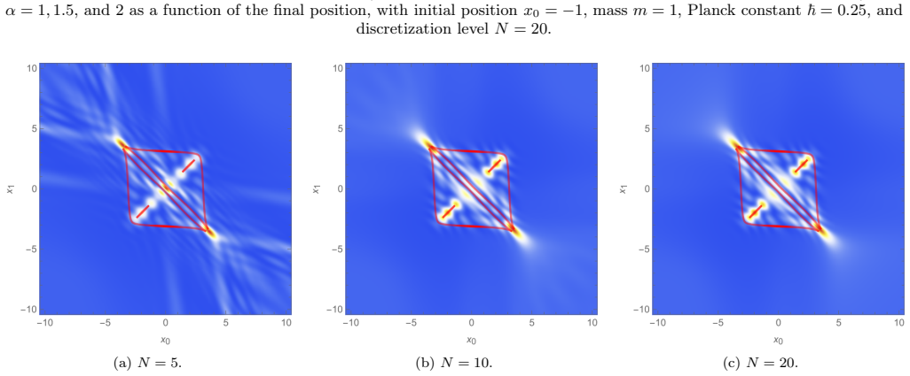
alpha = 1, 1.5, 2 for the truncated double well (Eq. 69)
- Lattice bounds and zero-padding size =
A = -50, B = 50 for the convergence test; padding described as problem-dependent (Section VI A)
- Gauss-Hermite quadrature order M =
not specified numerically
assumptions (5)
- domain assumption The lattice path integral with smooth analytic regularization is well defined and equivalent to an analytic deformation of the integrand or integration domain.
- domain assumption Cauchy's integral theorem justifies rotating the q_{n-1} contour by angle theta around q_s without crossing singularities of the analytically continued potential.
- ad hoc to paper For a potential with Hessian H V << 2 at infinity, the residual \delta I_n = I_n - \bar J_n decays at large |q_n| fast enough for FFT-based convolution on a padded lattice.
- domain assumption The discretized path integral G_N tends to the continuum propagator G as N tends to infinity for the potentials treated as functions.
- standard math The saddle maps xi_n and chi_n are invertible away from caustics, so the eikonal sums over real saddle points are valid.
Cite this review
Pith. "Pith review of Efficient evaluation of real-time path integrals." pith.science (2026). https://pith.science/paper/MIGM6QPV
@misc{pith2026250116323,
  author       = {Pith},
  title        = {Pith review of: Efficient evaluation of real-time path integrals},
  year         = {2026},
  howpublished = {\url{https://pith.science/paper/MIGM6QPV}},
  note         = {Machine review of arXiv:2501.16323}
}
read the original abstract
The Feynman path integral has revolutionized modern approaches to quantum physics. Although the path integral formalism has proven very successful and spawned several approximation schemes, the direct evaluation of real-time path integrals is still extremely expensive and numerically delicate due to its high-dimensional and oscillatory nature. We propose an efficient method for the numerical evaluation of the real-time world-line path integral for theories where the potential is dominated by a quadratic at infinity. This is done by rewriting the high-dimensional oscillatory integral in terms of a series of low-dimensional oscillatory integrals, that we efficiently evaluate with Picard-Lefschetz theory or approximate with the eikonal approximation. Subsequently, these integrals are stitched together with a series of fast Fourier transformations to recover the lattice regularized Feynman path integral. Our method directly applies to problems in quantum mechanics, the word-line quantization of quantum field theory, and quantum gravity.
Figures


Figures from the paper (8 more)



Reference graph
Works this paper leans on
-
[1]
First, approximate/evaluate the integralsJ2, . . . , JN on a regular lattice using either an explicit deformation of the integration contour or a saddle point approximation as discussed in section IIID. Alternatively, we can use the numerical implementation of Picard-Lefschetz theory for families of low-dimensional integrals presented in [15]
-
[2]
Next, stitch theJn’s together to evaluate the integralsI2, . . . , IN. Starting with I2(q2) = J2(q2) , (37) we evaluate the residualδI2 using the rule δIn(qn) = In(qn) − ¯Jn(qn) , (38) and find the next stepI3 using the iterative process In+1(qn+1) = Jn+1(qn+1) + F −1 h F δIn(qn)e− ia ℏ V (qn) e− iaℏk2 2m i , (39) with the fast Fourier transformationF and...
-
[3]
Upon normalizing In Gn(x1, x0, an) = ce− ia 2ℏ [V (x0)+V (x1)]In(x1) , (40) we obtain the discretized path integral forn = 1, . . . , N. This process simultaneously yields the discretized path integralGn for a lattice of propagation times and final positions forafixedinitialposition x0. Byrepeatingthisprocedureforalatticeofinitialpositions x0, weevaluatet...
-
[4]
Numerical evaluation For the numerical evaluation, deform the integration domain by rotating the contour around the saddle point of the kinetic termqs such that it is parametrized by γn−1(λ) = qs + eiθλ , (44) for λ ∈ Rd and some anglesθ ∈ [0, 2π)d. Letting qn−1 = γn−1(λ), the integral assumes the form Jn(qn) = c (n − 1)d/2 e im 2aℏ (qn −x0 )2 n +i(θ1+···...
-
[5]
For aqn outside these regions, the potentialP m V ( ¯q) is free of singularities (see fig
First find the singularities ofV in the complex plane and identify the convex hulls of the singularities in the upper and lower complex half-planes. For aqn outside these regions, the potentialP m V ( ¯q) is free of singularities (see fig. 1)
-
[6]
Next, deform the original integration domain into the complex planeCd while making sure that the deformed contour does not enter either of the two convex hulls (see fig. 1). This deformation suppresses the oscillations of the integrand for largeλ. The resulting integral can be efficiently numerically evaluated with standard integration techniques. Here we...
-
[7]
The eikonal approximation Alternatively, note how equation (42) scales with the number of discretization stepsN. As N increases, the effective reduced Planck constant, ℏef f= T ℏ mN n − 1 n , (47) 8 Re[qn] Im[qn] • • • • • • • • • • • x0 qn •qs FIG. 1: The proposed linear deformation of the integration domain in the complexqn plane. The convex hull (the s...
-
[8]
We define a regular lattice spatial lattice and approximate/evaluate theJn integrals on this lattice
Show all 57 references
-
[9]
This residual will generally vanish for large ∥qn∥
We evaluate the residual ofJn with respect to ¯Jn, defined asδJn = Jn − ¯Jn. This residual will generally vanish for large ∥qn∥
-
[10]
The required padding depends on the physical problem in question
As the convolutions will often grow beyond the size of the original lattice, we extend the lattice and pad the residual δJn with zeros. The required padding depends on the physical problem in question
-
[11]
When required, we downsize the result to match the original lattice
Next, we evaluate the convolutions using a series of fast Fourier transformations to obtain the discretized path integral GN. When required, we downsize the result to match the original lattice. In the examples presented in this paper, we evaluated theJn integrals both numeric...
-
[12]
R. P. Feynman,Feynman’s Thesis - a New Approach to Quantum Theory, edited by L. M. Brown (2005)
2005
-
[13]
R. P. Feynman, Reviews of Modern Physics20, 367 (1948)
1948
-
[14]
R. P. Feynman,QED. The strange theory of light and matter(1985)
1985
-
[15]
R. P. Feynman and A. R. Hibbs,Quantum mechanics and path integrals, International series in pure and applied physics (McGraw-Hill, New York, NY, 1965)
1965
-
[16]
Schulman,Techniques and Applications of Path Integration, Dover Books on Physics (Dover Publications, 2012)
L. Schulman,Techniques and Applications of Path Integration, Dover Books on Physics (Dover Publications, 2012)
2012
-
[17]
Kleinert, Path integrals in quantum mechanics, statistics, polymer physics, and financial markets; 3rd ed
H. Kleinert, Path integrals in quantum mechanics, statistics, polymer physics, and financial markets; 3rd ed. (World Scientific, River Edge, NJ, 2004) based on a Course on Path Integrals, Freie Univ. Berlin, 1989/1990
2004
-
[18]
Zee,Quantum field theory in a nutshell(2003)
A. Zee,Quantum field theory in a nutshell(2003)
2003
-
[19]
Polchinski,String Theory(1998)
J. Polchinski,String Theory(1998)
1998
-
[20]
G. W. Gibbons and S. W. Hawking,Euclidean quantum gravity(1993)
1993
-
[21]
Smit,Introduction to Quantum Fields on a Lattice(2002)
J. Smit,Introduction to Quantum Fields on a Lattice(2002)
2002
-
[22]
Turok, New Journal of Physics16, 063006 (2014), arXiv:1312.1772 [quant-ph]
N. Turok, New Journal of Physics16, 063006 (2014), arXiv:1312.1772 [quant-ph]
2014 arXiv
-
[23]
Feldbrugge, D
J. Feldbrugge, D. L. Jow, and U.-L. Pen, arXiv e-prints , arXiv:2309.12420 (2023), arXiv:2309.12420 [quant-ph]
2023 arXiv
-
[24]
Witten, arXiv e-prints , arXiv:1001.2933 (2010), arXiv:1001.2933 [hep-th]
E. Witten, arXiv e-prints , arXiv:1001.2933 (2010), arXiv:1001.2933 [hep-th]
2010 arXiv
-
[25]
E.Arnold, S.Gusein-Zade, andA.Varchenko, Singularities of Differentiable Maps, Volume 2: Monodromy and Asymptotics of Integrals, Modern Birkhäuser Classics (Birkhäuser Boston, 2012)
2012
-
[26]
Feldbrugge, U.-L
J. Feldbrugge, U.-L. Pen, and N. Turok, Annals of Physics451, 169255 (2023)
2023
-
[27]
Feldbrugge and N
J. Feldbrugge and N. Turok, arXiv e-prints , arXiv:2008.01154 (2020), arXiv:2008.01154 [gr-qc]
2020 arXiv
-
[28]
Feldbrugge, MNRAS520, 2995 (2023), arXiv:2010.03089 [astro-ph.CO]
J. Feldbrugge, MNRAS520, 2995 (2023), arXiv:2010.03089 [astro-ph.CO]
2023 arXiv
-
[29]
D. L. Jow, U.-L. Pen, and J. Feldbrugge, MNRAS525, 2107 (2023), arXiv:2204.12004 [astro-ph.HE]
2023 arXiv
-
[30]
Cristoforetti, F
M. Cristoforetti, F. Di Renzo, and L. Scorzato, Phys. Rev. D86, 074506 (2012), arXiv:1205.3996 [hep-lat]
2012 arXiv
-
[31]
Cristoforetti, F
M. Cristoforetti, F. Di Renzo, A. Mukherjee, and L. Scorzato, arXiv e-prints , arXiv:1312.1052 (2013), arXiv:1312.1052 [hep-lat]
2013 arXiv
-
[32]
Fujii, D
H. Fujii, D. Honda, M. Kato, Y. Kikukawa, S. Komatsu, and T. Sano, Journal of High Energy Physics2013, 147 (2013), arXiv:1309.4371 [hep-lat]. 19
2013 arXiv
-
[33]
Alexandru, G
A. Alexandru, G. Basar, P. F. Bedaque, G. W. Ridgway, and N. C. Warrington, Journal of High Energy Physics2016, 53 (2016)
2016
-
[34]
Alexandru, G
A. Alexandru, G. Başar, P. F. Bedaque, and N. C. Warrington, Phys. Rev. D96, 034513 (2017), arXiv:1703.02414 [hep-lat]
2017 arXiv
-
[35]
Fukuma and N
M. Fukuma and N. Umeda, Progress of Theoretical and Experimental Physics2017, 073B01 (2017), arXiv:1703.00861 [hep-lat]
2017 arXiv
-
[36]
Fukuma, N
M. Fukuma, N. Matsumoto, and N. Umeda, arXiv e-prints , arXiv:1912.13303 (2019), arXiv:1912.13303 [hep-lat]
2019 arXiv
-
[37]
Fukuma and N
M. Fukuma and N. Matsumoto, Progress of Theoretical and Experimental Physics2021, 023B08 (2021), arXiv:2012.08468 [hep-lat]
2021 arXiv
-
[38]
G.Fujisawa, J.Nishimura, K.Sakai, andA.Yosprakob,JournalofHighEnergyPhysics 2022,179(2022),arXiv:2112.10519 [hep-lat]
2022 arXiv
-
[39]
Nishimura, K
J. Nishimura, K. Sakai, and A. Yosprakob, Journal of High Energy Physics2023, 110 (2023), arXiv:2307.11199 [hep-th]
2023 arXiv
-
[40]
Nishimura, K
J. Nishimura, K. Sakai, and A. Yosprakob, Journal of High Energy Physics2024, 174 (2024), arXiv:2404.16589 [hep-lat]
2024 arXiv
-
[41]
Feldbrugge, J.-L
J. Feldbrugge, J.-L. Lehners, and N. Turok, Phys. Rev. D95, 103508 (2017), arXiv:1703.02076 [hep-th]
2017 arXiv
-
[42]
Chou and J
C.-Y. Chou and J. Nishimura, arXiv e-prints , arXiv:2407.17724 (2024), arXiv:2407.17724 [gr-qc]
2024 arXiv
-
[43]
Feldbrugge and N
J. Feldbrugge and N. Turok, Annals of Physics454, 169315 (2023), arXiv:2207.12798 [hep-th]
2023 arXiv
-
[44]
Klauder,A Modern Approach to Functional Integration, Applied and Numerical Harmonic Analysis (Birkhäuser Boston, 2010)
J. Klauder,A Modern Approach to Functional Integration, Applied and Numerical Harmonic Analysis (Birkhäuser Boston, 2010)
2010
-
[45]
When an integral diverges absolutely, R |f (x)|dx = ∞, the convergence of the integral R f (x)dx subtly depends on the regularization of the integral
-
[46]
J. R. Klauder, inA Garden of Quanta: Essays in Honor of Hiroshi Ezawa. Edited by ARAFUNE J ET AL. Published by World Scientific Publishing Co. Pte. Ltd, edited by J. Arafune and et al. (2003) pp. 55–76
2003
-
[47]
Thompson, Contemporary Physics52, 497 (2011)
I. Thompson, Contemporary Physics52, 497 (2011)
2011
-
[48]
Pöschl and E
G. Pöschl and E. Teller, Zeitschrift fur Physik83, 143 (1933)
1933
-
[49]
Rosen and P
N. Rosen and P. M. Morse, Physical Review42, 210 (1932)
1932
-
[50]
Kleinert and I
H. Kleinert and I. Mustapic, Journal of Mathematical Physics33, 643 (1992)
1992
-
[51]
Grosche and F
C. Grosche and F. Steiner,Handbook of Feynman Path Integrals, Handbook of Feynman Path Integrals No. v. 145 (Springer Berlin Heidelberg, 1998)
1998
-
[52]
Grosche and F
C. Grosche and F. Steiner, arXiv e-prints , hep-th/9302053 (1993), arXiv:hep-th/9302053 [hep-th]
1993 arXiv
-
[53]
Schulman, inFunctional integration and its applications(Oxford Univ
L. Schulman, inFunctional integration and its applications(Oxford Univ. Press London, 1975)
1975
-
[54]
S. A. Fulling and K. S. Güntürk, American Journal of Physics71, 55 (2003)
2003
-
[55]
Crank, P
J. Crank, P. Nicolson, and D. R. Hartree, Proceedings of the Cambridge Philosophical Society43, 50 (1947)
1947
-
[56]
De Raedt, Computer Physics Reports7, 1 (1987)
H. De Raedt, Computer Physics Reports7, 1 (1987)
1987
-
[57]
J. A. Wheeler, Annals of Physics2, 604 (1957). Appendix A: Stitching method for Gaussian initial state The solution of the Schrödinger equation can be written as the convolution of the initial state with the propagator. For completeness, we here develop the stitching method fo...
1957
Reviewed August 10, 2026 · model on record in the stance chip above.
Discussion (0). Continue with ORCID to comment.