REVIEW 3 major objections 3 minor 66 references
Training a data re-uploading quantum classifier with native control pulses instead of gate rotations yields ~80% test accuracy and far greater noise tolerance than the equivalent gate-based circuit, in simulations of a superconducting trans
Reviewed by Pith at T0; open to challenge. T0 means a machine referee read the full paper against a public rubric. the ladder, T0–T4 →
T0 review · deepseek-v4-flash
2026-08-03 17:03 UTC pith:MORLWXIE
load-bearing objection Plausible idea, but the main noise-resilience claim is unverified because the noise model's insertion rule is ambiguous. the 3 major comments →
Pulsed learning for quantum data re-uploading models
The pith
A machine-rendered reading of the paper's core claim, the machinery that carries it, and where it could break.
Core claim
The central claim is that replacing each parameterized gate in a data re-uploading QNN with a physically motivated pulse schedule—resonant single-qubit pulses flanked by virtual-Z rotations, and a single cross-resonance-inspired entangling pulse with trainable amplitude, phase, and detuning—yields a model that is at least as expressive and substantially more noise-tolerant than the gate-based original. In numerical simulation of a superconducting transmon processor using device-like coherence times and error rates, the pulse-based model achieves approximately 80% test accuracy across layer counts from 5 to 40, while the gate-based model saturates near 60%; and the pulse model retains roughly
What carries the argument
The key object is the pulse-level replacement of the trainable unitary blocks. Each single-qubit SU(2) becomes two virtual-Z rotations (error-free phase updates) around a resonant constant-amplitude pulse whose amplitude and phase are trainable. Each two-qubit entangling block is a single cross-resonance-style pulse with trainable amplitude, phase, and frequency detuning, able to modulate or suppress entanglement. A fidelity-based loss and a warm-started two-qubit initialization (starting from the trained one-qubit parameters) carry the training.
Load-bearing premise
The comparison assumes the simplified noise model charges each pulse a single error event with probabilities set by native gate errors; if noise is applied per Trotter-Suzuki slice instead of per physical pulse, the claimed pulse advantage could be an artifact.
What would settle it
Read the released simulation code to check where depolarizing, amplitude-damping, and phase-damping channels are applied relative to Trotter-Suzuki slices; then rerun the two-qubit 20-layer experiment with noise applied continuously over pulse duration. If the gate-based model then reaches about 80% test accuracy, the claimed pulse advantage is an artifact of the noise discretization.
If this is right
- Pulse-native training reduces the number of concatenated error-prone operations, so learning models can exploit more layers without immediately succumbing to noise.
- The roughly 80% test accuracy sustained up to depolarizing probability p≈0.1 gives near-term QML a larger usable noise budget than gate-based circuits.
- Because the methodology replaces arbitrary gates by native pulses, it can be applied to other variational QML architectures, not just data re-uploading.
- Pulse-level models overfit later as depth grows, indicating better generalization from the same amount of training data.
- The approach moves QML closer to the native control language of hardware, reducing calibration overhead in principle.
Where Pith is reading between the lines
- The fairness of the gate-versus-pulse comparison hinges on a simulation detail flagged in the paper's own footnote: pulses are Trotterized into 'dozens of gates,' and if noise is charged per Trotter slice rather than per physical pulse, the pulsed model is effectively a deeper noisy circuit and the reported advantage may be an artifact.
- A direct hardware experiment with real pulse schedules, where T1/T2 decay during each pulse duration is physically integrated, would be the cleanest test of whether the advantage survives outside the simplified Markovian noise model.
- The authors leave pulse-based data encoding to future work; making the encoding itself trainable could either widen the generalization gap or add noise-sensitive parameters, and is an obvious next step.
Editorial analysis
A structured set of objections, weighed in public.
Referee Report
Summary. The paper proposes a pulse-level formulation of data re-uploading quantum machine learning, replacing parameterized gate-based variational layers with native control pulses on a simulated transmon processor. Trainable parameters are moved into the pulse amplitudes, phases, and detunings, while the encoding blocks remain gate-based. The authors benchmark the pulse-based model against a gate-based counterpart on binary MNIST classification (digits 0 vs 8), using a two-qubit data re-uploading architecture with warm-start initialization. The central empirical claims are that the pulsed model achieves substantially higher test accuracy (~80% vs ~60%) and maintains this accuracy for depolarizing noise probability p up to about 0.1, whereas the gate-based model degrades sooner. Noise is modeled with amplitude damping, phase damping, and depolarizing channels parameterized from IBM Brisbane calibration data, with a separate depolarizing sweep in Fig. 6(b).
Significance. If the central claims hold, the paper would provide a concrete, hardware-aligned alternative to gate-based variational QML, with meaningful implications for noise-resilient model design on superconducting processors. The manuscript has several strengths: it uses publicly available device parameters, provides a code repository, includes a warm-start training procedure, and systematically studies both layer-count and noise-strength dependence. The generalization gap and the noise-resilience plateau are striking and potentially important. However, the validity of the empirical benchmark depends on whether the pulse and gate models are compared under genuinely equivalent noise conditions. The main weakness is that the noise insertion convention for the Trotterized pulse simulation is unspecified, and this ambiguity directly affects the paper's central conclusion. If the noise insertion is per Trotter slice, the reported pulse robustness is very surprising and may be an artifact; if it is per physical pulse, the comparison may not be at equivalent error strength. The learnable target states and the different two-qubit parameterizations also introduce possible confounds that need to be a
major comments (3)
- [Appendix B.3 and footnote 56] The central comparison in Fig. 6(b) requires that the pulse and gate models incur comparable error events. Appendix B.3 states that depolarizing, amplitude damping, and phase damping channels are applied after each electromagnetic control pulse or single-qubit gate, while footnote 56 states that each pulse is simulated via a Trotter-Suzuki decomposition into 'dozens of gates.' It is not specified whether noise channels are inserted per Trotter slice or per physical pulse. If noise is applied per slice, a single pulse suffers many error events, making the pulsed model a deep noisy circuit and the robustness at p≈0.1 implausible. If noise is applied per pulse, the per-event error strength and pulse duration are not calibrated to native gate errors. Please state the noise insertion points explicitly (ideally with a code snippet) and report the number of Trotter steps per pulse.
- [Section IV.C / Fig. 6(b)] The noise-sweep protocol is incompletely defined. The text says p is the probability of collapsing to the maximally mixed state and that all other noise parameters are held constant, but it does not say how p is applied in the pulsed simulation: per Trotter slice, per physical pulse, or per native gate. It also does not define 'equivalent noise conditions' operationally. If the pulsed model applies p once per physical pulse while the gate model applies it per gate, the comparison is not at matched error counts. Please specify the exact noise schedules for both models and, if necessary, rerun the sweep under matched error conventions.
- [Section IV.A / Eqs. (8)-(9)] The learnable target states |s0(θ,φ)> and |s1(θ,φ)> are introduced in the experimental setup and are used in the fidelity-based cost. It is not stated explicitly whether these target-state parameters are trained for both the gate-based and pulse-based models. If they are used only in the pulsed model, the test-accuracy gap in Fig. 6(a) could be explained by this extra trainable flexibility rather than by pulse-level training. If they are used in both models, this should be stated when the models are defined in Section III.
minor comments (3)
- [Fig. 6] Please clarify what the error bars represent and how they are computed over the five random seeds. The caption and text should state whether the plotted intervals are standard deviations, standard errors, or min/max ranges.
- [References] Reference [22] lists 'H. T. el al.' and is incomplete; reference [37] is missing a title; reference [55] is missing a title. Please fix these bibliographic entries.
- [Appendix B] Typo: 'quantum channelss' should be 'quantum channels.' Also, the notation in Eqs. (B2)-(B4) uses p, γ, and λ without explicitly connecting the depolarizing probability p to the device error rates described later; a brief summary of the mapping would improve readability.
Circularity Check
No equation-level circularity; mild construction-based circularity in the pulse noise model.
specific steps
-
other
[Appendix B.3 / footnote 56; load-bearing claim in Section IV.C / Fig. 6(b)]
"Specifically, depolarizing, amplitude damping, and phase damping channels are applied after each electromagnetic control pulse or single-qubit gate. ... On the code implementation, pulses are simulated using the Trotter-Suzuki approximation, with each pulse divided into dozens of gates."
The central noise-resilience claim is that the pulsed model retains ~80% test accuracy up to p≈0.1 while the gate model degrades sooner. The simulation generates this result by applying one noise channel per pulse, while footnote 56 says each pulse is internally a Trotter-Suzuki sequence of dozens of gates. If noise is applied per pulse, the pulse model is credited with fewer error events by construction, so the conclusion follows from the error-counting rule rather than from an independently calibrated pulse error model; if noise is applied per Trotter slice, the pulse model is a deeper noisy circuit and the advantage is not robust. The manuscript does not resolve this, making the central resilience comparison partly an artifact of the noise-insertion convention.
full rationale
The paper is an empirical benchmark rather than a first-principles derivation. The pulse ansatz in Eq. (7) and the fidelity cost in Eq. (10) are not defined in terms of each other, and no fitted parameter is renamed as a prediction. The self-citation to [44] for the underlying data re-uploading architecture is not load-bearing: the pulse-versus-gate comparison is independent of the architecture's provenance. The only mild circularity is localized to the construction of the noise simulation: the pulse model is treated as one error event per pulse even though a pulse is Trotter-decomposed into many gates, so the noise-resilience result in Fig. 6(b) partly reduces to how errors are counted. This is as much a calibration/correctness ambiguity as a circularity, but it is the one place where the claimed advantage is built into the comparison rather than independently demonstrated.
Axiom & Free-Parameter Ledger
free parameters (4)
- Per-layer single-qubit pulse parameters (Omega, gamma, nu1, nu2) =
trained on MNIST 0-vs-8 subset
- Per-layer two-qubit pulse parameters (amplitude, phase, detuning) =
trained
- Target state parameters theta and phi =
trained
- Pulse duration T and pulse shape s(t) =
fixed: sinusoidal constant amplitude; durations from Table I (1Q 300 ns, 2Q 660 ns)
axioms (5)
- domain assumption Driven transmon Hamiltonian under RWA, Eq. (A7)-(A9)
- domain assumption Dispersive elimination of the resonator and CR effective Hamiltonian, Eq. (A12)-(A14)
- domain assumption Markovian noise model: depolarizing, amplitude damping, phase damping, and SPAM channels applied independently after each operation
- ad hoc to paper Trotter-Suzuki decomposition faithfully represents pulse dynamics and noise is assigned in a physically meaningful way
- domain assumption PCA to 3 dimensions preserves enough MNIST information for the classification question
read the original abstract
While Quantum Machine Learning (QML) holds great potential, its practical realization on Noisy Intermediate-Scale Quantum (NISQ) hardware has been hindered by the limitations of variational quantum circuits (VQCs). Recent evidence suggests that VQCs suffer from severe trainability and noise-related issues, leading to growing skepticism about their long-term viability. However, the possibility of implementing learning models directly at the pulse-control level remains comparatively unexplored and could offer a promising alternative. In this work, we formulate a pulse-based variant of data re-uploading, embedding trainable parameters directly into the native system's dynamics. We benchmark our approach on a simulated superconducting transmon processor with realistic noise profiles. The pulse-based model consistently outperforms its gate-based counterpart, exhibiting higher test accuracy and improved generalization under equivalent noise conditions. Moreover, by systematically increasing noise strength, we show that pulse-level implementations retain higher fidelity for longer, demonstrating enhanced resilience to decoherence and control errors. These results suggest that pulse-native architectures, though less explored, may offer a viable and hardware-aligned path forward for practical QML in the NISQ era.
Figures



Reference graph
Works this paper leans on
-
[1]
The spectrum is har- monic, preventing isolation of a two level system
The Transmon Qubit Hamiltonian To understand transmon’s physics, we start with the LC cir- cuit, equivalent to a quantum harmonic oscillator with Hamil- tonian [19] ˆHLC = ˆQ2 2C + ˆΦ2 2L,(A1) where ˆQand ˆΦare conjugate operators. The spectrum is har- monic, preventing isolation of a two level system. To in- troduce anharmonicity, the linear inductor is ...
-
[2]
The qubit-field interaction can be modelled by the Hamiltonian [59] ˆH=− ω0 2 ˆσz −Ω ( eiωdtˆσ+ +e−iωdtˆσ−) =− ω0 2 ˆσz −Ω ( cos(ωdt)ˆσx−sin(ωdt)ˆσy )
Driven transmon: effective qubit Hamiltonian The control of the effective two-level system just described, can be addressed by adding an external microwave drive field, 10 capacitively coupled to the circuit. The qubit-field interaction can be modelled by the Hamiltonian [59] ˆH=− ω0 2 ˆσz −Ω ( eiωdtˆσ+ +e−iωdtˆσ−) =− ω0 2 ˆσz −Ω ( cos(ωdt)ˆσx−sin(ωdt)ˆσy...
-
[3]
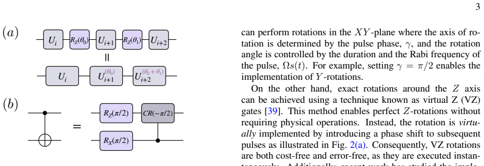
VirtualZgates While directZrotations can be performed via detuned pulses, a more efficient approach exploitsVirtualZ(VZ) gates [39]. These gates are implemented purely in software: they adjust the reference frame of the qubit rather than apply- ing a physical pulse, making them effectively instantaneous and error-free. A rotation about an arbitrary axis i...
-
[4]
Connecting transmon qubits Qubits must be connected to enable two-qubit operations. While many coupling schemes exist, a highly exploited ar- chitecture are the fixed frequency couplers, used in IBM de- vices [19], which avoid the need for tunable qubit frequencies or coupling elements. In general, capacitive coupling intro- duces an interaction term of t...
-
[5]
A convenient representation of these channels is theoperator- sum representation, also known as the Kraus representation
Quantum Channels and Kraus Operators Noise in quantum systems is typically described using the formalism ofquantum channels, which are completely posi- tive trace-preserving (CPTP) maps acting on density matrices. A convenient representation of these channels is theoperator- sum representation, also known as the Kraus representation. In this formalism, th...
-
[6]
Depolarizing Channel The depolarizing channel represents a stochastic process where the qubit state is replaced by the maximally mixed state with probabilityp
Superconducting Noise Contributions a. Depolarizing Channel The depolarizing channel represents a stochastic process where the qubit state is replaced by the maximally mixed state with probabilityp. For a single qubit, the Kraus operators are: K0 = √ 1−pI, K 1 = √p 3 ˆσX, K2 = √p 3 ˆσY, K 3 = √p 3 ˆσZ. (B2) Here,p∈[0,1]denotes the probability of a random ...
-
[7]
Modelling the IBM Brisbane Device To validate our model with realistic numerical simulations, we parameterize the noise channels described above using the specifications of the IBM Brisbane device. As the simulation of larger systems is computationally expensive, we restrict our study to two-qubit models, which are sufficiently complex to demonstrate the ...
-
[8]
A. B. Rashid and M. A. K. Kausik, Ai revolutionizing indus- tries worldwide: A comprehensive overview of its diverse ap- plications, Hybrid Advances7, 100277 (2024)
2024
-
[9]
S. S. Gill, O. Cetinkaya, S. Marrone, D. Claudino, D. Haunschild, L. Schlote, H. Wu, C. Ottaviani, X. Liu, S. P. Machupalli, K. Kaur, P. Arora, J. Liu, A. Farouk, H. H. Song, S. Uhlig, and K. Ramamohanarao, Quantum Computing: Vi- sion and Challenges, arXiv:2403.02240 (2024)
Pith/arXiv arXiv 2024
-
[10]
J. Biamonte, P. Wittek, N. Pancotti, P. Rebentrost, N. Wiebe, and S. Lloyd, Quantum machine learning, Nature549, 10.1038/nature23474 (2017)
-
[11]
Cerezo, G
M. Cerezo, G. Verdon, H.-Y . Huang, L. Cincio, and P. Coles, Challenges and opportunities in quantum machine learning, Nature Computational Science2(2022)
2022
-
[12]
Y . Du, X. Wang, N. Guo, Z. Yu, Y . Qian, K. Zhang, M.-H. Hsieh, P. Rebentrost, and D. Tao, Quantum machine learning: A hands-on tutorial for machine learning practitioners and re- searchers (2025), arXiv:2502.01146 [quant-ph]
Pith/arXiv arXiv 2025
-
[13]
Rebentrost, M
P. Rebentrost, M. Mohseni, and S. Lloyd, Quantum support vector machine for big data classification, Phys. Rev. Lett.113, 130503 (2014)
2014
-
[14]
Lloyd, M
S. Lloyd, M. Mohseni, and P. Rebentrost, Quantum principal component analysis, Nature Physics10, 631 (2014)
2014
-
[15]
Tang, Dequantizing algorithms to understand quantum ad- vantage in machine learning, Nature Reviews Physics4, 692 (2022)
E. Tang, Dequantizing algorithms to understand quantum ad- vantage in machine learning, Nature Reviews Physics4, 692 (2022)
2022
-
[16]
Y . Liu, S. Arunachalam, and K. Temme, A rigorous and ro- bust quantum speed-up in supervised machine learning, Nature Physics17, 1013 (2021)
2021
-
[17]
Preskill, Quantum Computing in the NISQ era and beyond, Quantum2, 10.22331/q-2018-08-06-79 (2018)
J. Preskill, Quantum Computing in the NISQ era and beyond, Quantum2, 10.22331/q-2018-08-06-79 (2018)
-
[18]
Benedetti, E
M. Benedetti, E. Lloyd, S. Sack, and M. Fiorentini, Parame- terized quantum circuits as machine learning models, Quantum Science and Technology4, 043001 (2019)
2019
-
[19]
Cerezo, A
M. Cerezo, A. Arrasmith, R. Babbush, S. C. Benjamin, S. Endo, K. Fujii, J. R. McClean, K. Mitarai, X. Yuan, L. Cin- cio, and P. J. Coles, Variational quantum algorithms, Nature Reviews Physics3, 625 (2021)
2021
-
[20]
A. Pérez-Salinas, A. Cervera-Lierta, E. Gil-Fuster, and J. I. Latorre, Data re-uploading for a universal quantum classifier, Quantum4, 10.22331/q-2020-02-06-226 (2020)
-
[22]
Y . Du, Z. Tu, X. Yuan, and D. Tao, Efficient measure for the expressivity of variational quantum algorithms, Phys. Rev. Lett. 128, 080506 (2022)
2022
-
[23]
Gil-Fuster, J
E. Gil-Fuster, J. Eisert, and C. Bravo-Prieto, Understanding quantum machine learning also requires rethinking generaliza- tion, Nature Communications15, 2277 (2024)
2024
-
[24]
J. Bowles, S. Ahmed, and M. Schuld, Better than classical? the subtle art of benchmarking quantum machine learning models, ArXivabs/2403.07059(2024)
Pith/arXiv arXiv 2024
-
[26]
P. Krantz, M. Kjaergaard, F. Yan, T. P. Orlando, S. Gustavsson, and W. D. Oliver, A quantum engineer’s guide to supercon- ducting qubits, Applied Physics Reviews6, 10.1063/1.5089550 (2019)
-
[27]
T. Alexander, N. Kanazawa, D. J. Egger, L. Capelluto, C. J. Wood, A. Javadi-Abhari, and D. C McKay, Qiskit pulse: programming quantum computers through the cloud with pulses, Quantum Science and Technology5, 10.1088/2058- 9565/aba404 (2020)
doi:10.1088/2058- 2058
-
[28]
K. N. Smith, G. S. Ravi, T. Alexander, N. T. Bronn, A. R. R. Carvalho, A. Cervera-Lierta, F. T. Chong, J. M. Chow, M. Cubeddu, A. Hashim, L. Jiang, O. Lanes, M. J. Otten, D. I. Schuster, P. Gokhale, N. Earnest, and A. Galda, Programming physical quantum systems with pulse-level control, Frontiers in PhysicsV olume 10 - 2022, 10.3389/fphy.2022.900099 (2022)
arXiv 2022
-
[29]
H. T. el al., On the Role of Controllability in Pulse-based Quan- tum Machine Learning Models, arXiv:2405.09135 (2024)
Pith/arXiv arXiv 2024
-
[30]
K. X. Wei, E. Magesan, I. Lauer, S. Srinivasan, D. F. Bo- gorin, S. Carnevale, G. A. Keefe, Y . Kim, D. Klaus, W. Lan- ders, N. Sundaresan, C. Wang, E. J. Zhang, M. Steffen, O. E. Dial, D. C. McKay, and A. Kandala, Hamiltonian engineering with multicolor drives for fast entangling gates and quantum 13 crosstalk cancellation, Phys. Rev. Lett.129, 060501 (2022)
2022
-
[31]
O. R. Meitei, B. T. Gard, G. S. Barron, D. P. Pappas, S. E. Economou, E. Barnes, and N. J. Mayhall, Gate-free state prepa- ration for fast variational quantum eigensolver simulations: ctrl-vqe (2021), arXiv:2008.04302 [quant-ph]
Pith/arXiv arXiv 2021
-
[32]
K. M. Sherbert, H. Amer, S. E. Economou, E. Barnes, and N. J. Mayhall, Parametrization and optimizability of pulse-level variational quantum eigensolvers, Phys. Rev. Appl.23, 024036 (2025)
2025
-
[33]
D. J. Egger, C. Capecci, B. Pokharel, P. K. Barkoutsos, L. E. Fischer, L. Guidoni, and I. Tavernelli, Pulse variational quan- tum eigensolver on cross-resonance-based hardware, Phys. Rev. Res.5, 033159 (2023)
2023
-
[34]
Y . Wang, Y . Ding, F. A. Cárdenas-López, and X. Chen, Pulse- based variational quantum optimization and metalearning in su- perconducting circuits (2024), arXiv:2407.12636 [quant-ph]
Pith/arXiv arXiv 2024
-
[35]
D. Meirom and S. H. Frankel, Pansatz: pulse-based ansatz for variational quantum algorithms, Frontiers in Quantum Science and Technology2, 10.3389/frqst.2023.1273581 (2023)
arXiv 2023
-
[36]
A. Melo, N. Earnest-Noble, and F. Tacchino, Pulse-efficient quantum machine learning, Quantum7, 1130 (2023)
2023
-
[37]
Z. Liang, H. Wang, J. Cheng, Y . Ding, H. Ren, Z. Gao, Z. Hu, D. S. Boning, X. Qian, S. Han, W. Jiang, and Y . Shi, Variational quantum pulse learning (2022), arXiv:2203.17267 [quant-ph]
Pith/arXiv arXiv 2022
-
[38]
Z. Liang, J. Cheng, Z. Song, H. Ren, R. Yang, K. Liu, P. Kogge, T. Li, Y . Ding, and Y . Shi, Towards advantages of parameterized quantum pulses (2024), arXiv:2304.09253 [quant-ph]
Pith/arXiv arXiv 2024
-
[39]
H.-X. Tao, X. Wang, and R.-B. Wu, On the design of expressive and trainable pulse-based quantum machine learning models (2025), arXiv:2508.05559 [quant-ph]
arXiv 2025
-
[41]
D’Alessandro,Introduction to Quantum Control and Dy- namics, 1st ed
D. D’Alessandro,Introduction to Quantum Control and Dy- namics, 1st ed. (Chapman and Hall/CRC, 2007)
2007
-
[42]
R. Acharya and A. et al, Quantum error correction below the surface code threshold, Nature 10.1038/s41586-024-08449-y (2024)
-
[43]
Arute and K
F. Arute and K. A. et al, Quantum Supremacy using a Pro- grammable Superconducting Processor, Nature574(2019)
2019
-
[44]
Corporation, IBM Unveils Breakthrough 127-Qubit Quantum Processor (), accessed on: 2024-12-25
I. Corporation, IBM Unveils Breakthrough 127-Qubit Quantum Processor (), accessed on: 2024-12-25
2024
-
[46]
D. C. McKay, C. J. Wood, S. Sheldon, J. M. Chow, and J. M. Gambetta, Efficient Z gates for quantum computing, Physical Review A96, 10.1103/physreva.96.022330 (2017)
-
[47]
C. K. Long and C. H. W. Barnes, From virtual z gates to virtual z pulses (2025), arXiv:2509.13453 [quant-ph]
arXiv 2025
-
[48]
Magesan and J
E. Magesan and J. M. Gambetta, Effective hamiltonian models of the cross-resonance gate, Phys. Rev. A101, 052308 (2020)
2020
-
[49]
Heya and N
K. Heya and N. Kanazawa, Cross-cross resonance gate, PRX Quantum2, 040336 (2021)
2021
-
[50]
Leone, S
L. Leone, S. F. Oliviero, L. Cincio, and M. Cerezo, On the prac- tical usefulness of the Hardware Efficient Ansatz, Quantum8, 1395 (2024)
2024
-
[51]
Rodriguez-Grasa, Y
P. Rodriguez-Grasa, Y . Ban, and M. Sanz, Neural quantum ker- nels: Training quantum kernels with quantum neural networks, Phys. Rev. Res.7, 023269 (2025)
2025
-
[52]
D. J. Egger, J. Mare ˇcek, and S. Woerner, Warm-starting quan- tum optimization, Quantum5, 479 (2021)
2021
-
[53]
R. Puig, M. Drudis, S. Thanasilp, and Z. Holmes, Variational quantum simulation: A case study for understanding warm starts, PRX Quantum6, 010317 (2025)
2025
-
[54]
H. Mhiri, R. Puig, S. Lerch, M. S. Rudolph, T. Chotibut, S. Thanasilp, and Z. Holmes, A unifying account of warm start guarantees for patches of quantum landscapes (2025), arXiv:2502.07889 [quant-ph]
Pith/arXiv arXiv 2025
-
[55]
H.-X. Tao, J. Hu, and R.-B. Wu, Unleashing the expres- sive power of pulse-based quantum neural networks (2024), arXiv:2402.02880 [quant-ph]
Pith/arXiv arXiv 2024
-
[56]
N. Earnest, C. Tornow, and D. J. Egger, Pulse-efficient cir- cuit transpilation for quantum applications on cross-resonance- based hardware, Physical Review Research3, 10.1103/phys- revresearch.3.043088 (2021)
doi:10.1103/phys- 2021
-
[57]
J. R. McClean, S. Boixo, V . N. Smelyanskiy, R. Babbush, and H. Neven, Barren plateaus in quantum neural network training landscapes, Nature Communications9, 10.1038/s41467-018- 07090-4 (2018)
-
[58]
Easom-Mccaldin, A
P. Easom-Mccaldin, A. Bouridane, A. Belatreche, and R. Jiang, On Depth, Robustness and Performance Using the Data Re- Uploading Single-Qubit Classifier, IEEE Access9(2021)
2021
-
[59]
J. R. McClean, S. Boixo, V . N. Smelyanskiy, R. Babbush, and H. Neven, Barren plateaus in quantum neural network training landscapes, Nature Communications9, 4812 (2018)
2018
-
[60]
K. e. a. Williams, Quantification of Robustness, Leakage, and Seepage for Composite and Adiabatic Gates on Modern NISQ Systems, Intelligent Computing3, 10.34133/icomputing.0069 (2024)
-
[61]
J. Gil-Lopez, M. Santandrea, and et al, Improved non-linear devices for quantum applications, New Journal of Physics23, 10.1088/1367-2630/ac09fd (2021)
-
[62]
Corporation, Brisbane Quantum Computer Description (), ac- cessed on: 2024-12-12
I. Corporation, Brisbane Quantum Computer Description (), ac- cessed on: 2024-12-12
2024
-
[63]
The gradient for each gate is computed dur- ing training, making even a simple QNN computationally in- tensive
On the code implementation, pulses are simulated using the Trotter-Suzuki approximation, with each pulse divided into dozens of gates. The gradient for each gate is computed dur- ing training, making even a simple QNN computationally in- tensive
-
[64]
Georgopoulos, C
K. Georgopoulos, C. Emary, and P. Zuliani, Modeling and sim- ulating the noisy behavior of near-term quantum computers, Phys. Rev. A104, 062432 (2021)
2021
-
[65]
Deng, The MNIST Database of Handwritten Digit Images for Machine Learning Research, IEEE Signal Processing Mag- azine29(2012)
L. Deng, The MNIST Database of Handwritten Digit Images for Machine Learning Research, IEEE Signal Processing Mag- azine29(2012)
2012
-
[66]
Corporation,Qiskit notebook(2024) Chap
I. Corporation,Qiskit notebook(2024) Chap. Introduction to Transmon Physics
2024
-
[67]
E. Magesan and J. M. Gambetta, Effective Hamiltonian mod- els of the cross-resonance gate, Physical Review A101, 10.1103/physreva.101.052308 (2020)
-
[68]
K. Georgopoulos, C. Emary, and P. Zuliani, Modeling and sim- ulating the noisy behavior of near-term quantum computers, Physical Review A104, 10.1103/physreva.104.062432 (2021)
-
[69]
T. Piskor, M. Schöndorf, M. Bauer, D. Smith, T. Ayral, S. Pogorzalek, A. Auer, and M. Papi ˇc, Simulation and bench- marking of real quantum hardware (2025), arXiv:2508.04483 [quant-ph]
Pith/arXiv arXiv 2025
-
[70]
M. A. Nielsen and I. L. Chuang,Quantum Computation and Quantum Information: 10th Anniversary Edition(Cambridge University Press, 2010)
2010
discussion (0)
Sign in with ORCID, Apple, or X to comment. Anyone can read and Pith papers without signing in.