REVIEW 4 major objections 4 minor 29 references
Imaging at the quantum limit with convolutional neural networks
T0 review · 4 major / 4 minor · reviewed 2026-08-15 · deepseek-v4-flash
Pith's one-line read A convolutional neural network trained on noisy images can reach the minimum variance allowed by quantum mechanics for coherent-state illumination, even when the image's parametric form is unknown.
desk verdict Interesting simulation, but the central claim that a U-Net learns to become the optimal estimator does not follow: comparing a biased estimator's MSE to a variance-only bound is not an optimality test. read the letter →
The pith
A machine-rendered reading of the paper's core claim, the machinery that carries it, and where it could break.
The reading
What carries the argument
The quantum Fisher information matrix (QFIM) carries the argument: for a coherent probe with mean photon number $\bar{N}$ and uniform spatial profile, its elements are $F_{ij}=4\bar{N}\int |\alpha(x,y)|^2 (\partial\phi/\partial\theta_i)(\partial\phi/\partial\theta_j)\,dx\,dy$. Inverting $F$ gives the QCRB covariance matrix, and Jacobian propagation turns these parameter variances into a pixel-wise image-variance map that can be compared directly with the U-Net's mean-squared error. The U-Net's convolutional skip connections are the estimator machinery that learns the correlations encoded in $F$ from data alone.
What would settle it
Compute the network's squared bias separately by averaging its predictions over many independent noise realizations for a fixed true image and subtracting the true image; if the squared bias is a substantial fraction of the mean-squared error, the apparent saturation of the quantum Cramér-Rao bound would not by itself establish that the network is the optimal unbiased estimator.
Extended reading notes
Core claim
The central claim is that a 2D U-Net trained on simulated coherent-state measurements learns, for each image domain it is trained on, the minimum-variance estimator allowed by quantum metrology. For images built from superimposed linear and radial sinusoids with 3–11 parameters, the authors compute the quantum Fisher information matrix $F_{ij}=4\bar{N}\int dx\,dy\,|\alpha(x,y)|^2\, \partial\phi/\partial\theta_i\, \partial\phi/\partial\theta_j$, invert it to get the QCRB covariance $\Sigma \ge F^{-1}$, and propagate those parameter variances through the image Jacobian to obtain pixel-wise variance maps. Across five sinusoid families and mean photon numbers inside the training range, the network's average MSE fluctuates around this QCRB variance; outside the trained photon-number range the MSE diverges from the bound. For unparameterized natural images, the per-pixel shot-noise limit is routinely surpassed, which the authors attribute to the network using inter-pixel correlations, so the proper comparison for such images would require a correlated quantum Fisher information matrix.
Load-bearing premise
The comparison assumes that the network's mean-squared error, which includes bias, can be compared directly to a variance-only bound; if the network is biased, the bound match would not establish that it is the optimal estimator.
Editorial extensions
If this is right
- Within the range of photon numbers used in training, the network's reconstruction error saturates the quantum Cramér-Rao bound, so it can serve as an optimal estimator for coherent-state imaging without an explicit parametric model.
- Outside the trained photon-number range, the match degrades, indicating that the learned optimality is specific to the training domain.
- Apparent violations of the standard quantum and Heisenberg limits on natural images are explained by inter-pixel correlations; the correct benchmark for correlated images is a correlated quantum Fisher information matrix, not a per-pixel variance sum.
- The same training methodology could be applied to nonclassical probe states, where the relevant bound is the Heisenberg limit rather than the shot-noise limit.
Reading between the lines
- Editorial inference: because mean-squared error includes squared bias, a biased network could show MSE below the QCRB without being the optimal unbiased estimator; separating bias and variance over many noise realizations would tell whether the saturation is genuine.
- Editorial inference: the agreement between MSE and QCRB could be used as a diagnostic: a network that saturates the bound for a given image family has likely internalized the true generative parameters; monitoring this gap during training may reveal when a model has learned the data-generating process.
- Editorial inference: if saturation is a general property of convolutional architectures, then alternative encoder-decoder models should also reach the bound on the same image families; this prediction is directly testable.
Signed reviews
Editorial analysis
A structured set of objections, weighed in public.
Referee Report
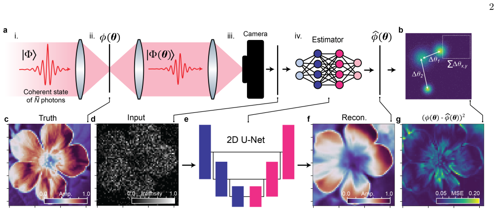
Summary. The paper trains 2D U-Net models to reconstruct 64x64 intensity images from simulated coherent-state measurements corrupted by Poisson shot noise. For unparameterized natural images of flowers, it compares the pixelwise mean-squared error (MSE) of reconstructions to the standard quantum limit (SQL) and Heisenberg limit (HL) and reports that the average MSE can fall below both. For parameterized images built from superposed sinusoids, the authors compute the quantum Fisher information matrix and quantum Cramér-Rao bound (QCRB) for the image parameters, propagate the bound to pixel variances, and report that the network's MSE closely tracks the QCRB across several sinusoid families and photon-number ranges. The paper concludes that convolutional neural networks can learn to become optimal estimators at the ultimate precision limits.
Significance. The central claim, if established, would be notable: it would show that a generic learned estimator can saturate the quantum Fisher-information limit for coherent-state imaging without being given the parametric model, which would be practically useful for low-light imaging. The manuscript has strengths: it provides code, tests multiple parametric families, uses on-the-fly test images outside the validation set, and checks settings outside the training photon-number range. However, the comparison underpinning the claim is currently invalid because the QCRB is a variance bound for unbiased estimators, while the network is biased and the reported metric is MSE. The paper contains the relevant admission itself in Section II, so the gap is not an external subtlety. The result is therefore not yet supported, but the deficiency is addressable with additional analysis rather than being fatal to the research direction.
major comments (4)
- [Section III, Eq. (1); Figs. 3-4] The QCRB bounds the covariance matrix of an unbiased estimator of θ; it does not bound the mean-squared error of a biased estimator. Because MSE = variance + squared bias (as the authors note in Section II), an MSE numerically equal to the QCRB is consistent with an estimator whose variance lies above the bound and whose bias compensates. The manuscript provides no measurement of the network's bias, no bias-corrected bound (e.g., a van Trees-type bound), and no comparison with a known optimal unbiased estimator such as maximum likelihood for these sinusoid models. Without one of these, the headline claim that the network becomes the optimal estimator does not follow.
- [Section III; Supplementary Table II] The network is trained on parameter values drawn from the same bounded random distribution used at test time, so its predictions can exploit prior information about the parameter distribution. The QCRB, by contrast, is computed for each fixed true θ and does not include prior information. A biased/regularized estimator can therefore achieve an MSE below the per-θ variance bound. To support the optimality claim, the authors should either evaluate the bias for fixed θ values, report parameter-estimation errors rather than image-space MSE, or compare against the maximum-likelihood estimator on the same test instances.
- [Figs. 3-4; Section III] The claim that the MSE 'reaches' the QCRB is supported only by visual proximity of curves and images; no quantitative measure of agreement (e.g., ratio of MSE to QCRB with standard errors) or statistical test is reported. Given the central role of this equality, the manuscript should quantify the discrepancy over the tested parameter samples and photon numbers, including error bars on the Monte Carlo MSE estimates.
- [Abstract; Section II; Figs. 2] The abstract's statement that average MSE for flower images can 'surpass' the SQL and reach the HL is not a valid comparison. The SQL and HL are variance bounds for unbiased pixel-wise estimators, while the reported quantity is the MSE of a biased model that exploits spatial correlations and smoothness priors. The authors themselves identify correlations in Section II, and the Discussion correctly cautions that the naive pixel-wise comparison is not appropriate; however, the abstract and conclusion retain the overclaim. These claims should be reworded to avoid implying that a classical measurement has beaten the Heisenberg limit.
minor comments (4)
- [Introduction] The phrase 'a natural questions arises' is a typo and should read 'a natural question arises.'
- [Section III and Fig. 3 caption] The text says the three example rows in Fig. 3 correspond to Nbar = 250, 1000, and 4000, while the figure caption says Nbar = 100, 1000, and 10000; the inconsistency should be corrected.
- [Supplementary Eq. (A1)] Equation (A1) has an unmatched parenthesis in the linear-sinusoid term; the closing parenthesis for 'sin' is missing.
- [Code Availability] The paper should specify the exact commit or version of the GitHub repository used for the reported results, and ideally provide a data-generation seed, to make the numerical claims reproducible.
Circularity Check
No circularity: the QCRB is an external bound and the U-Net comparison is empirical; the bias caveat is a validity issue, not a circular reduction.
full rationale
The derivation chain is not circular. The QCRB is an external benchmark taken from Villegas et al. [18] and is computed from the known parametric form of the sinusoid images and the coherent-state probe, with no dependence on the U-Net weights or outputs. The network's MSE is evaluated on independently generated Poisson-noise frames and compared with that bound; the comparison is empirical and the network could have failed to reach the bound. Self-citations to ref. [7] supply the U-Net architecture and the SSIM/GDL loss terms, but those are methodological inputs, not the quantum-limit claim; the central result is not a restatement of any prior work by these authors. The paper's own admission that NNs are typically biased estimators means the MSE-versus-QCRB comparison is a statistical-validity concern (MSE includes squared bias while the QCRB bounds variance only), so an MSE equal to the bound does not by itself prove unbiased optimality. That concern affects the strength of the physical conclusion but is not a circular reduction: no equation of the paper defines the predicted quantity in terms of the fitted quantity or identifies the bound with the training objective. Consequently, no circular step is present.
Assumptions & free parameters
free parameters (1)
- Sinusoid parameter sampling ranges =
a in [0,1], omega in [0.5/npix, 4/npix], phi,beta in [-pi,pi], x0,y0 in [-npix/2,npix/2]
assumptions (4)
- domain assumption Each pixel's detected photon number follows a Poisson distribution with mean equal to the true intensity N(x,y).
- domain assumption The illumination amplitude is uniform across the image, |alpha(x,y)|^2 = 1.
- domain assumption The quantum Fisher information matrix for a coherent state probe is F_ij = 4N integral |alpha|^2 (dphi/dtheta_i)(dphi/dtheta_j), following Villegas et al. [18].
- standard math Pixel-wise variance of the reconstructed image is obtained by propagating the parameter covariance Sigma through the Jacobian of phi(x,y;theta).
Cite this review
Pith. "Pith review of Imaging at the quantum limit with convolutional neural networks." pith.science (2026). https://pith.science/paper/MRUCP3VH
@misc{pith2026250613488,
  author       = {Pith},
  title        = {Pith review of: Imaging at the quantum limit with convolutional neural networks},
  year         = {2026},
  howpublished = {\url{https://pith.science/paper/MRUCP3VH}},
  note         = {Machine review of arXiv:2506.13488}
}
read the original abstract
Deep neural networks have been shown to achieve exceptional performance for computer vision tasks like image recognition, segmentation, and reconstruction or denoising. Here, we evaluate the ultimate performance limits of deep convolutional neural network models for image reconstruction, by comparing them against the standard quantum limit set by shot-noise and the Heisenberg limit on precision. We train U-Net models on images of natural objects illuminated with coherent states of light, and find that the average mean-squared error of the reconstructions can surpass the standard quantum limit, and in some cases reaches the Heisenberg limit. Further, we train models on well-parameterized images for which we can calculate the quantum Cram\'er-Rao bound to determine the minimum possible measurable variance of an estimated parameter for a given probe state. We find the mean-squared error of the model predictions reaches these bounds calculated for the parameters, across a variety of parameterized images. These results suggest that deep convolutional neural networks can learn to become the optimal estimators allowed by the laws of physics, performing parameter estimation and image reconstruction at the ultimate possible limits of precision for the case of classical illumination of the object.
Figures


Figures from the paper (1 more)

Reference graph
Works this paper leans on
-
[1]
Deep residual learning for image recognition,
K. He, X. Zhang, S. Ren, and J. Sun, “Deep residual learning for image recognition,” (2015), arXiv:1512.03385 [cs.CV]
arXiv 2015
-
[2]
J. Deng, W. Dong, R. Socher, L.-J. Li, K. Li, and L. Fei- Fei, in2009 IEEE Conference on Computer Vision and Pattern Recognition(2009) pp. 248–255
work page 2009
-
[3]
Z.-Q. Zhao, P. Zheng, S.-T. Xu, and X. Wu, IEEE Trans- actions on Neural Networks and Learning Systems30, 3212 (2019)
work page 2019
-
[4]
U-net: Con- volutional networks for biomedical image segmentation,
O. Ronneberger, P. Fischer, and T. Brox, “U-net: Con- volutional networks for biomedical image segmentation,” (2015), arXiv:1505.04597 [cs.CV]
arXiv 2015
-
[5]
J. Lequyer, R. Philip, A. Sharma, W.-H. Hsu, and L. Pel- letier, Nature Machine Intelligence4, 953 (2022)
work page 2022
-
[6]
G. Wang, J. C. Ye, and B. De Man, Nature Machine Intelligence2, 737 (2020)
work page 2020
-
[7]
A. H. Proppe, G. Thekkadath, D. England, P. J. Bustard, F. Bouchard, J. S. Lundeen, and B. J. Sussman, APL Machine Learning2, 036110 (2024)
work page 2024
-
[8]
A. H. Proppe, K. L. K. Lee, C. L. Cortes, M. Saif, D. B. Berkinsky, T. Sverko, W. Sun, J. Cassidy, M. Zamkov, T. Kim, E. Jang, S. K. Gray, B. A. McGuire, and M. G. Bawendi, Phys. Rev. B106, 045425 (2022)
work page 2022
Show all 29 references
-
[9]
A. H. Proppe, K. L. K. Lee, A. E. K. Kaplan, M. Gin- terseder, C. J. Krajewska, and M. G. Bawendi, Phys. Rev. Lett.131, 053603 (2023)
2023
-
[10]
Abdolghader, A
P. Abdolghader, A. Ridsdale, T. Grammatikopoulos, G. Resch, F. L´ egar´ e, A. Stolow, A. F. Pegoraro, and I. Tamblyn, Opt. Express29, 34205 (2021)
2021
-
[11]
Image restora- tion using very deep convolutional encoder-decoder networks with symmetric skip connections,
X.-J. Mao, C. Shen, and Y.-B. Yang, “Image restora- tion using very deep convolutional encoder-decoder networks with symmetric skip connections,” (2016), arXiv:1603.09056 [cs.CV]
2016 arXiv
-
[12]
Ahmed, C
S. Ahmed, C. S´ anchez Mu˜ noz, F. Nori, and A. F. Kockum, Phys. Rev. Lett.127, 140502 (2021)
2021
-
[13]
Hermosa, C
N. Hermosa, C. Rosales-Guzm´ an, S. F. Pereira, and J. P. Torres, Opt. Lett.39, 299 (2014)
2014
-
[14]
J. R. Hervas, L. L. S´ anchez-Soto, A. Z. Goldberg, Z. Hradil, and J. ˇReh´ aˇ cek, Phys. Rev. A110, 033716 (2024)
2024
-
[15]
K. A. G. Bonsma-Fisher, W.-K. Tham, H. Ferretti, and A. M. Steinberg, New Journal of Physics21, 093010 (2019)
2019
-
[16]
Tsang, R
M. Tsang, R. Nair, and X.-M. Lu, Phys. Rev. X6, 031033 (2016)
2016
-
[17]
Polino, M
E. Polino, M. Valeri, N. Spagnolo, and F. Sciarrino, AVS Quantum Science2, 024703 (2020), https://pubs.aip.org/avs/aqs/article- pdf/doi/10.1116/5.0007577/19738916/024703 1 online.pdf
2020 doi
-
[18]
Villegas, M
A. Villegas, M. H. M. Passos, S. F. Pereira, and J. P. Torres, Phys. Rev. A109, 032617 (2024)
2024
-
[19]
Giovannetti, S
V. Giovannetti, S. Lloyd, and L. Maccone, Phys. Rev. Lett.96, 010401 (2006)
2006
-
[20]
A survey on universal approximation theorems,
M. T. Augustine, “A survey on universal approximation theorems,” (2024), arXiv:2407.12895 [cs.LG]
2024 arXiv
-
[21]
A. M. Sch¨ afer and H. G. Zimmermann, inArtificial Neu- ral Networks – ICANN 2006, edited by S. D. Kollias, A. Stafylopatis, W. Duch, and E. Oja (Springer Berlin Heidelberg, Berlin, Heidelberg, 2006) pp. 632–640
2006
-
[22]
Nilsback and A
M.-E. Nilsback and A. Zisserman, inIndian Conference on Computer Vision, Graphics and Image Processing (2008)
2008
-
[23]
R. R. Selvaraju, M. Cogswell, A. Das, R. Vedantam, D. Parikh, and D. Batra, International Journal of Com- puter Vision128, 336–359 (2019). 8
2019
-
[24]
Paszke, S
A. Paszke, S. Gross, F. Massa, A. Lerer, J. Bradbury, G. Chanan, T. Killeen, Z. Lin, N. Gimelshein, L. Antiga, A. Desmaison, A. Kopf, E. Yang, Z. DeVito, M. Rai- son, A. Tejani, S. Chilamkurthy, B. Steiner, L. Fang, J. Bai, and S. Chintala, inAdvances in Neural Informa- tion P...
2019
-
[25]
Adam: A method for stochastic optimization,
D. P. Kingma and J. Ba, “Adam: A method for stochastic optimization,” (2017), arXiv:1412.6980 [cs.LG]. 9 Appendix A: Supplementary materials
2017 arXiv
-
[26]
For further information about the model architecture, see ref
Model training and hyperparameters The deep learning stack was implemented using PyTorch [24] and PyTorch Lightning, with weight updates performed using the Adam optimizer [25]; code and values for the data generation, hyperparameters, training, and evaluation pipeline can be ...
-
[27]
Details for simulating noisy frames can be found in ref
Datasets and data generation For the un-parameterized images of flowers, we trained our models on images of the flowers from the Oxford102 dataset [22]. Details for simulating noisy frames can be found in ref. [7]. For the parameterized images of sinusoids, we generated 64,000...
-
[28]
First, we calculate the Jacobian, which is a vector of partial derivatives of the functionfwith respect to the parametersθ 1,θ 2,θ 3: J(x1,x 2) = ∂f ∂θ1 ∂f ∂θ2 ∂f ∂θ3
Quantum Fisher information matrix calculations Here we demonstrate how the pixel-wise QCRB variances were calculated for the parameterized images. First, we calculate the Jacobian, which is a vector of partial derivatives of the functionfwith respect to the parametersθ 1,θ 2,θ...
-
[29]
S1: Histograms for the pixel values at pixel (32, 32) (top row) and (32, 1) (bottom row), for 100, 500, and 1000 images, with Gaussian fits to the distributions
Supporting figures FIG. S1: Histograms for the pixel values at pixel (32, 32) (top row) and (32, 1) (bottom row), for 100, 500, and 1000 images, with Gaussian fits to the distributions. 13 FIG. S2: (a) Training loss, (b) validation loss, and (c) MSE loss (from the validation d...
Reviewed August 15, 2026 · model on record in the stance chip above.
Discussion (0). Continue with ORCID to comment.