Dynamic Symmetric Point Tracking: Tackling Non-ideal Reference in Analog In-memory Training

Jindan Li; Quan Xiao; Tayfun Gokmen; Tianyi Chen; Zhaoxian Wu

REVIEW 3 major objections 5 minor 11 references

Dynamic Symmetric Point Tracking: Tackling Non-ideal Reference in Analog In-memory Training

T0 review · 3 major / 5 minor · reviewed 2026-08-02 · deepseek-v4-flash

Challenge this review Re-run · record.json Download PDF Read on arXiv ↗

Pith's one-line read The paper proves that a dynamic tracker can estimate the analog device symmetric point during training, achieving SGD-level convergence while cutting SP-calibration pulse count from O(δ^-2 + δ^-1/Δw_min) to O(δ^-2).

desk verdict The zero-shifting pulse-complexity bound is a real result worth citing, but the dynamic-tracking theorem rests on an unvalidated coordinate-wise gradient lower bound, and the experiments test a different algorithm than the one proved. read the letter →

arxiv 2602.21321 v2 pith:NKHWLZKW submitted 2026-02-24 cs.LG cs.ARmath.OC

Quan Xiao , Jindan Li , Zhaoxian Wu , Tayfun Gokmen , Tianyi Chen This is my paper

classification cs.LGcs.ARmath.OC

keywords analogin-memorycomputingsymmetricpointestimationzero-shiftingresiduallearningupdateasymmetrypulsecomplexitydynamictrackingchoppingandfiltering

verification ladder T0 review T1 audit T2 compute T3 formal

The pith

A machine-rendered reading of the paper's core claim, the machinery that carries it, and where it could break.

The reading

Analog in-memory training suffers from update asymmetry that drags weights toward a device-specific symmetric point (SP). Existing methods assume this SP is known and spend many pulses calibrating it to zero; this paper gives the first bound showing that reaching SP-error δ by zero-shifting costs N = O(δ^-1 Δw_min^-1) pulses, so finer devices make calibration more expensive. The paper then proposes RIDER, which leaves the SP unknown and tracks it during training using a digital moving average of a residual device's state. Under strong convexity and a coordinate-wise lower bound on gradient magnitude, RIDER converges at O(κ1κ2^5/√K) + Θ(Δw_min), matching standard SGD, and needs only O(δ^-2) pulses total. An enhanced chopping/filtering variant, E-RIDER, accelerates tracking and is validated on MNIST and CIFAR-100.

What carries the argument

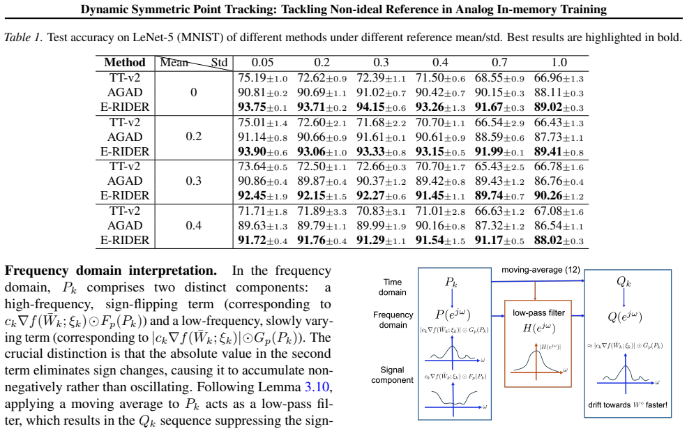
The central mechanism is the decomposition of each pulse response into a symmetric component F and an asymmetric component G, together with the observation that the residual device's update contains a term −α|∇f|⊙G_p(P_k) that always points toward the SP. A digital moving average amplifies this SP-attraction (Lemma 3.5), and the moving average acts as a low-pass filter from P to Q (Lemma 3.10). E-RIDER adds a random chopper sign c_k so the objective-descent component becomes high-frequency while the SP-drift component remains low-frequency, letting the filter extract the drift faster. Assumption 3.6, a coordinate-wise Rayleigh-type lower bound on expected absolute gradient, supplies the cont

What would settle it

Run RIDER with deterministic gradients (σ=0) on a device with nonzero SP: Assumption 3.6 is violated, and the predicted behavior is that Q_k stops approaching W⋄ and the training error floor exceeds Θ(Δw_min). Alternatively, log the coordinate-wise expected absolute gradient during training; if any coordinate falls below C⋆ before P_k reaches W⋄, the descent of φ(P_k) in Lemma E.3 changes sign. A pulse-count measurement would also settle it: for Δw_min=10^-4 and target δ≫Δw_min, RIDER should reach target loss with O(δ^-2) pulses while the two-stage zero-shifting baseline needs an additional O(

Watch

Extended reading notes

Core claim

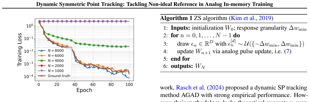
The paper models each analog pulse as a scaled intended update plus an asymmetric drift toward a device-specific symmetric point W⋄ where the asymmetric response G(W⋄)=0. It proves that the standard zero-shifting calibration requires N = O(δ^-1 Δw_min^-1) pulses to reach SP-error δ, so higher-precision devices pay more calibration pulses. It then introduces RIDER: a residual device P is updated by an analog rule whose |gradient| term always pushes P toward W⋄, while a digital moving average Q_{k+1} = (1−η)Q_k + ηP_{k+1} stays closer to W⋄ and supplies the compensation. Theorem 3.7 shows that with strongly convex objectives and step sizes α = Θ(1/√K), β = Θ(αγμ), η = Θ(αμ), the averaged error

Load-bearing premise

The proof needs every coordinate of the stochastic gradient to have expected absolute value at least C⋆ ≥ 4√2 σ/μ (q_max/q_min)^(3/2) at every step (Assumption 3.6); if any coordinate's gradient is too small, the negative term that drives the residual device toward the symmetric point disappears and the convergence argument collapses.

Editorial extensions

If this is right

For high-precision devices, the pulse cost of reaching training accuracy δ drops from O(δ^-2 + δ^-1/Δw_min) to O(δ^-2), removing the inverse-granularity calibration bottleneck.
Analog training with unknown, nonzero symmetric point matches the O(1/√K) SGD rate, with only the unavoidable Θ(Δw_min) granularity floor.
The compensation sequence Q_k lives digitally, so the W device needs no extra analog calibration; the SP is tracked on the fly rather than measured beforehand.
E-RIDER's chopping and filtering separate the objective-descent signal from the SP-drift signal in frequency, accelerating tracking without changing the descent direction.
The Θ(Δw_min) error floor means the limiting precision is device response granularity, not reference offset or calibration error.

Reading between the lines

Editorial extensions of the paper, not claims the author makes directly.

Because the contraction relies on Assumption 3.6, the strongest version of the result applies only in regimes with sufficient stochastic gradient noise; a noiseless or near-stationary gradient would leave P without a driving force toward the SP. This suggests the guarantees are about training dynamics, not about SP estimation in isolation.
The last-iterate bound for monotone response functions indicates the 1/Δw_min scaling is intrinsic to alternating-pulse zero-shifting, so the dynamic-tracking gain should persist for linear, exponential, and other monotone device models beyond the averaged analysis.
A natural testable extension is to let the SP drift slowly during training (device aging or temperature effects) and check whether the moving average Q_k tracks it; the fixed-point analysis suggests it would, but the paper's theorems assume a static W⋄.
The chopper probability p introduces a practical trade-off: the ablation shows a small p improves accuracy, but a large p would inject high-frequency noise into the descent; an adaptive p schedule is an obvious follow-up.

Share X Bluesky LinkedIn Reddit HN

Editorial analysis

A structured set of objections, weighed in public.

Desk editor's note, referee report, and a circularity audit.

Desk Editor's Note

read the letter

The reader's take is about right, and the stress-test note lands. This paper has one solid, genuinely new result: Theorem 2.2, the first explicit pulse-complexity bound for the zero-shifting algorithm, with the inverse-linear dependence on Δw_min that Figure 1b empirically confirms. That alone is worth something. The RIDER idea — tracking the symmetric point during training instead of paying a big calibration bill up front — is a natural and useful direction, and the low-pass-filter view of the moving average in Lemma 3.10 is a nice way to explain why chopping helps.

The soft spots are real and they are in the theory. Assumption 3.6 is not mild. It demands a coordinate-wise lower bound on E|∇f(·;ξ)| for every coordinate and every iteration, with a constant that scales like σ/μ times a device-condition factor. That fails exactly where the theory needs it most: near stationary points, or whenever the gradient estimator is deterministic in some coordinate. The proof of Lemma E.3 uses it to manufacture the negative descent term that drives P_k toward the SP, so without it Theorem 3.7 does not go through. The paper does not validate this assumption on any device model or simulate a regime where it is violated. That is load-bearing, not cosmetic.

There is also a theory–experiment gap. The theorem covers Algorithm 2 (RIDER, p=0), but the experiments use E-RIDER with a tuned chopper probability and a residual scale γ that are not analyzed. Figure 4's pulse-cost comparison depends on an assumed pulse length BL=5, which is a free parameter, and the paper ships no code or data. The "same rate as SGD" phrasing also overstates things a bit — the constants are κ1κ2^5 and there is a Θ(Δw_min) floor.

None of this is fatal. The ZS complexity result stands on its own, and the dynamic-tracking idea is worth developing. What the paper needs is an honest treatment of Assumption 3.6: either verify it on the AIHWKit device models, weaken it, or state clearly that Theorem 3.7 is conditional on a noise-regime assumption. It also needs experiments on RIDER itself, not just E-RIDER.

I would send this to peer review. A good referee can separate the citable ZS result from the shakier tracking theorem, and the authors seem competent to address the issues. It is a conditional accept in my view, not a reject.

Referee Report

3 major / 5 minor

Summary. This paper studies analog in-memory computing (AIMC) training under update asymmetry caused by device-specific symmetric points (SPs). It provides a convergence and pulse-complexity analysis of the standard zero-shifting (ZS) SP-estimation algorithm, proposes RIDER, a residual-learning algorithm with dynamic SP tracking, and an enhanced variant E-RIDER using chopping and filtering. It proves an O(κ1κ2^5/√K)+Θ(Δw_min) convergence bound for RIDER under Assumption 3.6 and derives a pulse-complexity advantage for dynamic tracking versus two-stage residual learning with ZS. Experiments on the AIHWKit simulator with MNIST and CIFAR-100 show that E-RIDER outperforms TT-v2 and AGAD.

Significance. The paper addresses a real and under-theorized problem: SP calibration cost in analog training. The ZS pulse-complexity characterization (Theorem 2.2) is a useful first step, and the idea of tracking the SP during training is timely. The proofs are detailed, with explicit condition-number dependence, and the appendices contain substantial supplementary material. However, the central convergence result rests on an unvalidated and, at stationary points, false coordinate-wise lower-bound assumption, and the experiments test only the empirically-enhanced E-RIDER, not the RIDER algorithm that is the subject of the theorem. If Assumption 3.6 can be justified or replaced with a weaker, validated condition, the contribution would be significant; in its current form the main dynamic-tracking claim is not established.

major comments (3)

[Section 3.1, Assumption 3.6; used in Lemma E.3 (Appendix E.4)] Assumption 3.6 is load-bearing and unvalidated. In Lemma E.3 (Eq. (100)) the lower bound E_{ξ_k}[|∇f(Ḡ_k;ξ_k)|_d] ≥ C⋆ is used to produce the negative term −(αC⋆/2)∥G_p(P_k)∥², which is the only descent mechanism for φ(P_k) and hence the only driver of SP tracking in Theorem 3.7. The assumption requires the expected absolute gradient to be bounded below in every coordinate at every iteration; this is not implied by Assumptions 3.2–3.4 and fails at stationary points or for deterministic full-batch gradients, where E|∇f_d|=0. The claimed magnitude C⋆ ≥ 4√2σ/μ (q_max/q_min)^{3/2} is restrictive for ill-conditioned objectives (μ≪1). The paper's justification that analog noise makes it mild (Section 3.1) is an assertion, not a validation; no device data or simulator trace is provided. This weakens the central claim.
[Section 4 and Appendix F.4] Experiments validate E-RIDER, not the algorithm covered by Theorem 3.7. Section 4 says RIDER is a special case of E-RIDER with p=0, but all experiments use the best-tuned chopper probability p>0 (Appendix F.4 shows p=0 is substantially worse). Theorem 3.7 proves convergence for Algorithm 2 (p=0), not Algorithm 3; no convergence theorem is given for E-RIDER. Thus the experimental results do not directly test the theoretical contribution. Either provide a convergence analysis (or at least a formal argument) for E-RIDER, or run RIDER (p=0) in the same settings so the effect of chopping is separated from the core tracking mechanism.
[Figure 4 (Section 4) and Corollary 3.9] Figure 4 does not validate Corollary 3.9. Corollary 3.9 compares RIDER with two-stage Residual Learning+ZS, whereas Figure 4 compares E-RIDER with TT-v2+ZS. The training pulse count is computed as epochs×⌈data size/B⌉×BL with BL=5, a free parameter not obtained from hardware; the result may change with BL. Also the theoretical pulse complexity is order-level, whereas the plot uses a specific cost model. Please report measured pulse counts from the simulator or show sensitivity of the comparison to BL and batch size.

minor comments (5)

[Introduction, Section 2.1] In the introduction, 'decomposing q+(w) and q−(w) into asymmetric component and an asymmetric component' should read 'symmetric component and an asymmetric component'. In Definition 2.1, 'Positive-definiteness' is a misnomer; the condition q_min >0 is a positivity/boundedness condition.
[Equation (14)] The metric E_K contains O(·) terms inside the expectation; using big-O inside an expectation is informal. Please replace with explicit constants or a defined norm.
[Theorem 3.7 statement] The condition C⋆ ≥ 4√2σ/μ (q_max/q_min)^{3/2} appears in the theorem but not in Assumption 3.6. Clarify whether this is an additional assumption or a consequence of other conditions; it is used in the proof to choose C2.
[Appendix C.4, Theorem C.4] The condition 'µ_q < 1/(3µ_q Δw_min)' is dimensionally inconsistent; it should likely be 'µ_q < 1/(3Δw_min)' or similar. Please correct.
[Figure 4 caption] The caption says 'hatched bars indicate the training cost computed as epochs×⌈data size/B⌉×BL' but BL is not defined in the caption. Define BL and state the batch size B explicitly.

Circularity Check

0 steps flagged · score 0.0 of 10

No significant circularity: RIDER's guarantees follow from stated assumptions and the analog-update model, not from fitted predictions or self-citation chains.

full rationale

The paper's central derivations are self-contained given the stated device and optimization assumptions. Theorem 2.2 is obtained by telescoping a potential-function descent for the zero-shifting update (7), with the O(1/(N Δw_min)) + Θ(Δw_min) bound following algebraically from the per-pulse magnitude and the bounded response functions; it involves no fitted parameter renamed as a prediction. Theorem 3.7 builds a Lyapunov function from the update rules (11)-(12) and proves sufficient descent using Lemmas E.1-E.3; the SP-tracking term in Lemma E.3 is produced directly by the −α|∇f|⊙G_p(P_k) term in the P-update together with Assumption 3.6, not by assuming the conclusion. Corollary 3.9 is arithmetic combination of the two theorems. The paper does rely on the authors' prior residual-learning model and on lemmas from Wu et al. (2025), but those are parameter-free modeling/technical inputs that do not contain the dynamic-tracking result; the prior work assumes a zero SP, whereas the present theorem addresses unknown nonzero SP, so the contribution is not a restatement. The strongest caveat is that Assumption 3.6 (coordinate-wise lower bound on E|∇f|) is strong and unvalidated, and Lemma 3.5's angle condition is asserted rather than proven, but these are correctness/rigor concerns about assumptions, not circular reductions of the claimed result to its inputs.

Assumptions & free parameters 3 free parameters · 7 assumptions · 0 invented entities

The main proof rests on standard smoothness/convexity assumptions plus two device-specific assumptions (bounded response, discretization-error scaling) and one paper-specific assumption (coordinate-wise lower bound on |∇f|, Assumption 3.6). The experimental accuracy claims depend on tuned hyperparameters and the AIHWKit simulator, so the central result is supported only modulo these assumptions.

free parameters (3)

E-RIDER residual scale γ = 0.1
Tuned manually; controls the weight of the residual term in W̄ and SP tracking. Appears in all E-RIDER runs (Tables 3-5). The theory only requires γ=Θ(1), not this specific value.
E-RIDER chopper probability p = 0.05 (input chop prob) for Table 1/2; 0.2 for Figure 4
Best-tuned over a sweep (Appendix F.4, Fig 5). p=0 gives worse performance, small p improves accuracy. The theory is for Algorithm 2/RIDER (p=0), not for E-RIDER with chopping.
Pulse length BL in Figure 4 pulse-cost calculation = 5
Used to convert training epochs into total pulse cost (epochs × ⌈data size/B⌉ × BL). Affects the reported total pulse cost for all methods and is a hardware-independent assumption.

assumptions (7)

standard math Assumption 3.1: f is L-smooth
Standard in optimization; used in Lemma E.1 and throughout the proof.
standard math Assumption 3.2: stochastic gradients are unbiased with bounded variance σ²
Standard SGD assumption; used in Lemma E.1 and E.3.
domain assumption Assumption 3.3: f is μ-strongly convex
Needed for the closed form P*(W,Q)=Q+(W*−W)/γ and for the convergence metric. Experiments use nonconvex networks, so this is a restriction on the theory.
domain assumption Assumption 3.4: discretization error b_k has zero mean and Var[b_k]=Θ(αΔw_min)
Borrowed from Li et al. 2025 (same research group); device-specific and not independently validated in this paper.
ad hoc to paper Assumption 3.6: E|∇f(W̄_k;ξ_k)|_d ≥ C⋆ with C⋆ ≥ 4√2 σ/μ (qmax/qmin)^(3/2) in every coordinate
Introduced here to force the negative SP-descent term in Lemma E.3. Strong and unvalidated; fails at stationary points with noiseless gradients. See weakest_assumption.
domain assumption Definition 2.1: q±(w) ∈ [qmin, qmax] and differentiable
Excludes saturating response functions where q±→0 at conductance bounds; needed for the boundedness and Lipschitz arguments in Theorem 2.2 and Lemma A.2.
domain assumption Model assumes coordinate-wise decoupled response functions and a unique SP W⋄
The update model in (2) is coordinate-wise and G(W⋄)=0 is assumed to have a unique zero; otherwise convergence of P_k to W⋄ is not guaranteed. Not stated as a separate assumption.

how reviews work

0 comments

Cite this review

Pith. "Pith review of Dynamic Symmetric Point Tracking: Tackling Non-ideal Reference in Analog In-memory Training." pith.science (2026). https://pith.science/paper/NKHWLZKW

@misc{pith2026260221321,
  author       = {Pith},
  title        = {Pith review of: Dynamic Symmetric Point Tracking: Tackling Non-ideal Reference in Analog In-memory Training},
  year         = {2026},
  howpublished = {\url{https://pith.science/paper/NKHWLZKW}},
  note         = {Machine review of arXiv:2602.21321}
}

read the original abstract

Analog in-memory computing (AIMC) performs computation directly within resistive crossbar arrays, offering an energy-efficient platform to scale large vision and language models. However, non-ideal analog device properties make the training on AIMC devices challenging. In particular, its update asymmetry can induce a systematic drift of weight updates towards a device-specific symmetric point (SP), which typically does not align with the optimum of the training objective. To mitigate this bias, most existing works assume the SP is known and pre-calibrate it to zero before training by setting the reference point as the SP. Nevertheless, calibrating AIMC devices requires costly pulse updates, and residual calibration error can directly degrade training performance. In this work, we present the first theoretical characterization of the pulse complexity of SP calibration and the resulting estimation error. We further propose a dynamic SP estimation method that tracks the SP during model training, and establishes its convergence guarantees. In addition, we develop an enhanced variant based on chopping and filtering techniques from digital signal processing. Numerical experiments demonstrate both the efficiency and effectiveness of the proposed method.

Figures

Figures reproduced from arXiv: 2602.21321 by the authors.

**Figure 1.** Trade-off between SP estimation accuracy and pulse cost for ZS algorithm. (a) For each N, we obtain per-cell SP estimates on a 512×512 array, and compute the mean and standard deviation across all cells. We plot the offsets of these statistics relative to the ground truth. (b) As ∆wmin decreases, achieving a target accuracy (e.g., ≤ 1% relative mean error) needs substantially more pulses. training process can also p… view at source ↗

**Figure 2.** Training loss on MNIST (LeNet-5, TT-v1 (Gokmen & Haensch, 2020)) using ground-truth SP and SPs estimated with different numbers of pulses N via zero-shifting Algorithm 1. C4) Numerical experiments validate the effectiveness and efficiency of the E-RIDER for simultaneous SP tracking and model training. With a more accurate SP estimation, the proposed method is able to improve the analog training accuracy in neural … view at source ↗

**Figure 3.** Chopping and filtering via moving average. on CIFAR-100 by training a ResNet-18 with the fully connected layer and the last residual block implemented in analog. All experiments are implemented in the AIHWKit simulator (Rasch et al., 2021). Note that RIDER is a special case of E-RIDER with p = 0. As shown in the Appendix F.4, using a small p > 0 yields a clear improvement in training performance, so we use E-RIDER… view at source ↗

Figures from the paper (2 more)

**Figure 4.** Figure 4: (Left) total pulse cost to reach the target training loss 0.2 on LeNet-5 (MNIST) across different number of states settings. Solid bars indicate the number of pulses using ZS algorithm, while hatched bars indicate the training cost computed as epochs×⌈data size/B⌉× BL,…

**Figure 5.** Figure 5: Test accuracy of E-RIDER on MNIST-FCN after 50 epochs under different input chopper probabilities p [PITH_FULL_IMAGE:figures/full_fig_p033_5.png]

Discussion (0). Sign in to comment.

Reference graph

Works this paper leans on

11 extracted references · 5 linked inside Pith

[1]

In practice, however, the SP of an analog device is usually determined experimentally by applying alternating positive and negative update pulses until the weight converges

Hyperparameter TT-v2 AGAD E-RIDER Units in mini-batch \ True True Transfer frequency (transfer every) 1.0 1.0 1.0 Transfer columns (transfer columns) True True True Self-transfer (no self transfer) True True True Reads per transfer (n reads per transfer) 1 1 1 Input chopping (in chop prob) \ 0.1 0.05 Input chopper random (in chop random) \ False False Out...

2024
[2]

and Wang, M

Ghadimi, S. and Wang, M. Approximation methods for bilevel programming.arXiv preprint arXiv:1802.02246,

arXiv
[4]

Comparison of E-RIDER, Residual Learning/TT-v2 and AGAD The proposed E-RIDER has a similar form of AGAD (Rasch et al., 2023)

B.2. Comparison of E-RIDER, Residual Learning/TT-v2 and AGAD The proposed E-RIDER has a similar form of AGAD (Rasch et al., 2023). However, AGAD uses the gradient ∇f(W k;ξ k) that are solely computed on the main array Wk. Instead, E-RIDER computes gradient on a mixed weight ¯Wk =W k + γck(Pk −Q k) so that achieves better performance in simulation. The key...

2023
[7]

Llama: Open and efficient foundation lan- guage models.arXiv preprint arXiv:2302.13971,

Touvron, H., Lavril, T., Izacard, G., Martinet, X., Lachaux, M.-A., Lacroix, T., Rozi`ere, B., Goyal, N., Hambro, E., Azhar, F., et al. Llama: Open and efficient foundation lan- guage models.arXiv preprint arXiv:2302.13971,

arXiv
[8]

With a slight abuse of notation, we also define the pseudo-inverse of a vectorW∈R D asW † :=diag(W) †

(19) By definition, the pseudo-inverse satisfies U U†V=U †U Vfor any diagonal matrix U∈R D and any matrix V∈R D. With a slight abuse of notation, we also define the pseudo-inverse of a vectorW∈R D asW † :=diag(W) †. Weighted norm.For a weightM∈R D +, the weighted norm∥ · ∥M ofW∈R D is defined by ∥W∥ M := vuut DX d=1 [M] d[W] 2 d = q W ⊤Diag(M)W(20) 12 Dyn...

2025
[10]

18 Dynamic Symmetric Point Tracking: Tackling Non-ideal Reference in Analog In-memory Training D.2

On the other hand, letting cos(Pk+1 − W ⋄, Pk+1 −Q k) := cosθ, we have ∥Qk −W ⋄∥2 =∥P k+1 −W ⋄∥2 +∥P k+1 −Q k∥2 −2∥P k+1 −W ⋄∥∥Pk+1 −Q k∥cosθ.(48) Plugging (48) into (47), we get ∥Qk+1 −W ⋄∥2 =∥P k+1 −W ⋄∥2 + (1−η) 2∥Pk+1 −Q k∥2 −2(1−η)∥P k+1 −W ⋄∥∥Pk+1 −Q k∥cosθ Sincecosθ >0implies∥P k+1 −Q k∥ ̸= 0, then choosing1> η >max n 1− 2∥Pk+1−W ⋄∥cosθ ∥Pk+1−Qk∥ ,...

2016
[2016]

J., Gokmen, T., Ando, T., Miyazoe, H., Kim, J.-J., Rozen, J., and Kim, S

Kim, H., Rasch, M. J., Gokmen, T., Ando, T., Miyazoe, H., Kim, J.-J., Rozen, J., and Kim, S. Zero-shifting technique for deep neural network training on resistive cross-point arrays.arXiv preprint arXiv:1907.10228,

arXiv 1907
[2018]

D., Dhariwal, P., Neelakantan, A., Shyam, P., Sastry, G., Askell, A., et al

Brown, T., Mann, B., Ryder, N., Subbiah, M., Kaplan, J. D., Dhariwal, P., Neelakantan, A., Shyam, P., Sastry, G., Askell, A., et al. Language models are few-shot learners. Advances in neural information processing systems, 33: 1877–1901,

1901

Show all 11 references

[2019]

In- memory training on analog devices with limited conduc- tance states via multi-tile residual learning.arXiv preprint arXiv:2510.02516,

Li, J., Wu, Z., Liu, G., Gokmen, T., and Chen, T. In- memory training on analog devices with limited conduc- tance states via multi-tile residual learning.arXiv preprint arXiv:2510.02516,
[2021]

J., Carta, F., Fagbohungbe, O., and Gokmen, T

Rasch, M. J., Carta, F., Fagbohungbe, O., and Gokmen, T. Fast offset corrected in-memory training.arXiv preprint arXiv:2303.04721,

arXiv
[2022]

A Two- Timescale Framework for Bilevel Optimization: Com- plexity Analysis and Application to Actor-Critic.arXiv preprint:2007.05170,

9 Dynamic Symmetric Point Tracking: Tackling Non-ideal Reference in Analog In-memory Training Hong, M., Wai, H.-T., Wang, Z., and Yang, Z. A Two- Timescale Framework for Bilevel Optimization: Com- plexity Analysis and Application to Actor-Critic.arXiv preprint:2007.05170,

2007 arXiv

Pith tools

Reviewed August 2, 2026 · model on record in the stance chip above.

[1] [1]

In practice, however, the SP of an analog device is usually determined experimentally by applying alternating positive and negative update pulses until the weight converges

Hyperparameter TT-v2 AGAD E-RIDER Units in mini-batch \ True True Transfer frequency (transfer every) 1.0 1.0 1.0 Transfer columns (transfer columns) True True True Self-transfer (no self transfer) True True True Reads per transfer (n reads per transfer) 1 1 1 Input chopping (in chop prob) \ 0.1 0.05 Input chopper random (in chop random) \ False False Out...

2024

[2] [2]

and Wang, M

Ghadimi, S. and Wang, M. Approximation methods for bilevel programming.arXiv preprint arXiv:1802.02246,

arXiv

[3] [4]

Comparison of E-RIDER, Residual Learning/TT-v2 and AGAD The proposed E-RIDER has a similar form of AGAD (Rasch et al., 2023)

B.2. Comparison of E-RIDER, Residual Learning/TT-v2 and AGAD The proposed E-RIDER has a similar form of AGAD (Rasch et al., 2023). However, AGAD uses the gradient ∇f(W k;ξ k) that are solely computed on the main array Wk. Instead, E-RIDER computes gradient on a mixed weight ¯Wk =W k + γck(Pk −Q k) so that achieves better performance in simulation. The key...

2023

[4] [7]

Llama: Open and efficient foundation lan- guage models.arXiv preprint arXiv:2302.13971,

Touvron, H., Lavril, T., Izacard, G., Martinet, X., Lachaux, M.-A., Lacroix, T., Rozi`ere, B., Goyal, N., Hambro, E., Azhar, F., et al. Llama: Open and efficient foundation lan- guage models.arXiv preprint arXiv:2302.13971,

arXiv

[5] [8]

With a slight abuse of notation, we also define the pseudo-inverse of a vectorW∈R D asW † :=diag(W) †

(19) By definition, the pseudo-inverse satisfies U U†V=U †U Vfor any diagonal matrix U∈R D and any matrix V∈R D. With a slight abuse of notation, we also define the pseudo-inverse of a vectorW∈R D asW † :=diag(W) †. Weighted norm.For a weightM∈R D +, the weighted norm∥ · ∥M ofW∈R D is defined by ∥W∥ M := vuut DX d=1 [M] d[W] 2 d = q W ⊤Diag(M)W(20) 12 Dyn...

2025

[6] [10]

18 Dynamic Symmetric Point Tracking: Tackling Non-ideal Reference in Analog In-memory Training D.2

On the other hand, letting cos(Pk+1 − W ⋄, Pk+1 −Q k) := cosθ, we have ∥Qk −W ⋄∥2 =∥P k+1 −W ⋄∥2 +∥P k+1 −Q k∥2 −2∥P k+1 −W ⋄∥∥Pk+1 −Q k∥cosθ.(48) Plugging (48) into (47), we get ∥Qk+1 −W ⋄∥2 =∥P k+1 −W ⋄∥2 + (1−η) 2∥Pk+1 −Q k∥2 −2(1−η)∥P k+1 −W ⋄∥∥Pk+1 −Q k∥cosθ Sincecosθ >0implies∥P k+1 −Q k∥ ̸= 0, then choosing1> η >max n 1− 2∥Pk+1−W ⋄∥cosθ ∥Pk+1−Qk∥ ,...

2016

[7] [2016]

J., Gokmen, T., Ando, T., Miyazoe, H., Kim, J.-J., Rozen, J., and Kim, S

Kim, H., Rasch, M. J., Gokmen, T., Ando, T., Miyazoe, H., Kim, J.-J., Rozen, J., and Kim, S. Zero-shifting technique for deep neural network training on resistive cross-point arrays.arXiv preprint arXiv:1907.10228,

arXiv 1907

[8] [2018]

D., Dhariwal, P., Neelakantan, A., Shyam, P., Sastry, G., Askell, A., et al

Brown, T., Mann, B., Ryder, N., Subbiah, M., Kaplan, J. D., Dhariwal, P., Neelakantan, A., Shyam, P., Sastry, G., Askell, A., et al. Language models are few-shot learners. Advances in neural information processing systems, 33: 1877–1901,

1901