REVIEW 4 major objections 7 minor 6 references
Magnetization Current Simulation of High Temperature Bulk Superconductors Using A-V-A Formulation and Iterative Algorithm Method: Critical State Model and Flux Creep Model
T0 review · 4 major / 7 minor · reviewed 2026-08-14 · deepseek-v4-flash
Pith's one-line read An iterative load-step algorithm lets ANSYS simulate bulk superconductor magnetization in both critical-state and flux-creep models.
desk verdict A genuine, useful ANSYS workflow for trapped-field simulations, with solid flux-creep benchmarking but a critical-state validation that is partly hand-imposed rather than independently solved. read the letter →
The pith
A machine-rendered reading of the paper's core claim, the machinery that carries it, and where it could break.
The reading
What carries the argument
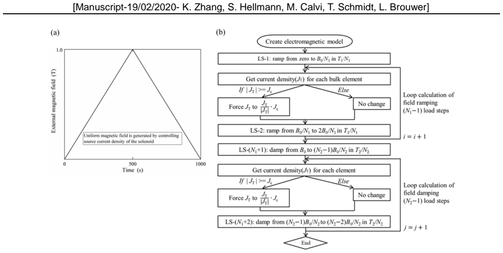
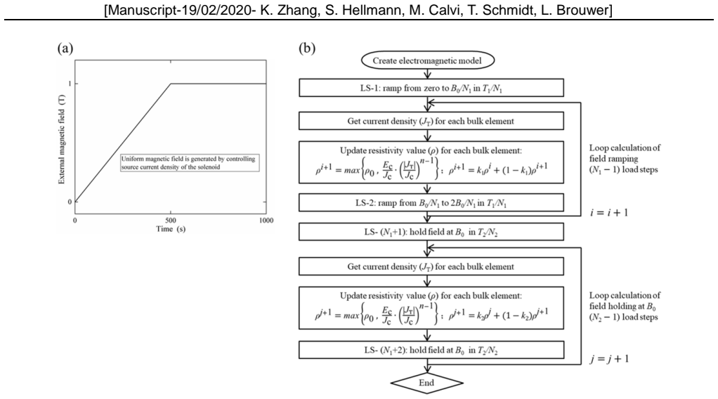
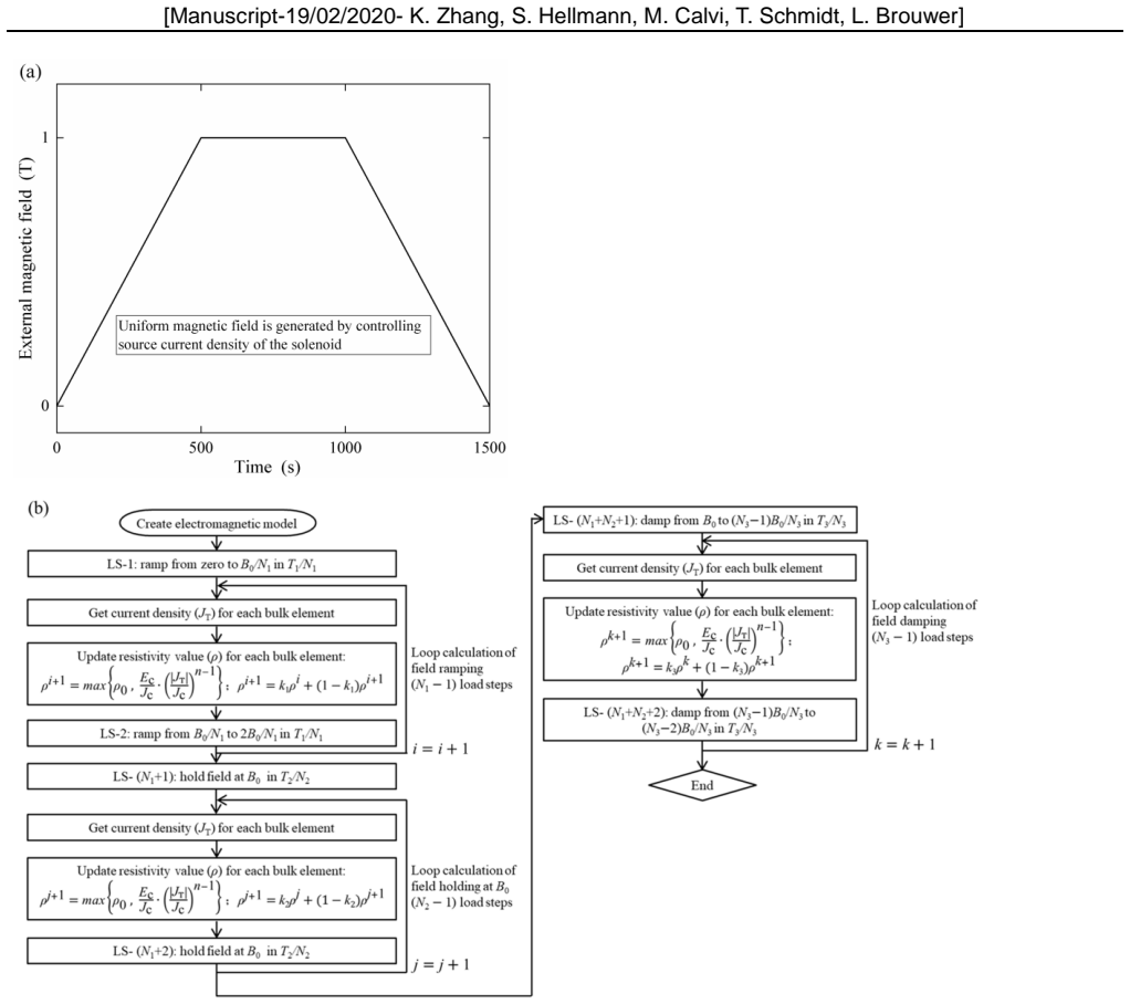
The carrying mechanism is the A-V-A formulation combined with an outer iterative loop. In superconductor regions the solver uses the magnetic vector potential $\mathbf{A}$ together with the electric scalar potential $V$, while non-superconductor regions use $\mathbf{A}$ alone, which shortens computation time. After each applied-field load step the method either clamps the trapped current density to $J_c$ using force commands (critical state model) or updates the resistivity with the E-J power law $\rho = \max\{\rho_0, (E_c/J_c)(|J|/J_c)^{n-1}\}$ and a mixing coefficient $k$ (flux creep model). For the field-descending branch of the critical state model, the method imposes the nodal voltage $V = -2\pi r \rho_0 J_c$ on penetrated elements to keep the inner-layer current from decaying while the outer layer reverses.
What would settle it
Run the same iterative loop on a pulsed-field magnetization (ramp to 1 T in about 50 ms) or on a rectangular tape stack, and compare the trapped-field profile and penetration depth against an H-formulation simulation or a magnetization measurement; any systematic front mismatch would show the clamping step distorts time-dependent penetration.
Extended reading notes
Core claim
The central claim is that magnetization currents in bulk superconductors can be computed by a load-step loop in which each step solves the A-V-A formulation (A-V in the superconductor, A-only elsewhere) and then directly enforces the constitutive law: set $|J| = J_c$ in penetrated elements for the critical state model, or update the element resistivity with $\rho = \max\{\rho_0, (E_c/J_c)(|J|/J_c)^{n-1}\}$ using a relaxation coefficient for the flux creep model. The paper reports good agreement with H-formulation results in COMSOL for a 25 mm diameter, 10 mm thick ReBCO disk in zero-field cooling, field cooling, and field reversal, and shows that the same loop can absorb ferromagnetic inserts, field-dependent $J_c(B)$, and strain-dependent $J_c(\varepsilon)$. It further claims practical advantages: adjustable computation time (about 2 to 3 seconds per load step), multi-frame restart analysis, and easy convergence even at large $n$-values.
Load-bearing premise
The method assumes that clamping the current density to $J_c$ after each load step, together with the node-voltage condition of Eq. (5), gives the same penetration dynamics as the true critical state model; the paper supports this only by matching one COMSOL disk profile.
Editorial extensions
If this is right
- A trapped-field magnet designer can run magnetization simulations in ANSYS with a freely chosen trade-off between accuracy and speed by setting the number of load steps.
- The same iterative loop handles ferromagnetic flux guides around the bulk, so realistic magnet assemblies can be modeled without changing the core algorithm.
- Because $J_c(B)$ and $J_c(\varepsilon)$ enter as per-element updates after each load step, the method can couple electromagnetic solving to mechanical stress analysis during the magnetization process.
- The restart capability means a multi-day simulation can be stopped and resumed after a workstation interruption without losing intermediate results.
- For the flux creep model, selecting a relaxation coefficient $k$ near 1 (for example 0.99) is necessary to keep the resistivity update stable; too-small $k$ (0.8 or 0.7) yields discontinuous current profiles.
Reading between the lines
- If the equivalence to H-formulation persists for multi-cycle or pulsed-field magnetization, the same clamping loop could turn any commercial eddy-current solver into a critical-state solver, removing the need for custom partial-differential-equation interfaces.
- The ad hoc node-voltage condition used during field descent is only justified by the single disk benchmark; a natural stress test is to compare the method against measured AC loss in a coil or stack, where repeated flux reversal exercises the inner-layer decay handling.
- The smoothing coefficients $k_1$-$k_3$ resemble numerical filters; a systematic study of their optimal values versus mesh size and time step would turn the current practical recipe into a calibrated convergence criterion.
Signed reviews
Editorial analysis
A structured set of objections, weighed in public.
Referee Report
Summary. This paper proposes an iterative algorithm method (IAM) embedded in ANSYS for simulating magnetization currents in disk-shaped ReBCO bulk superconductors. The method uses the A-V formulation in superconducting regions and the A-formulation elsewhere. For the critical-state model, after each load step the trapped current density in penetrated elements is forced to Jc; for the flux-creep model, element resistivities are updated according to the E-J power law with smoothing coefficients. The authors compare ZFC and FC results with COMSOL H-formulation simulations, report extensions to ferromagnetic inserts, Jc(B), and Jc(ε), and study the influence of load-step number, initial resistivity, ramping time, and updating coefficient.
Significance. If correct, the method offers a practical ANSYS-based alternative for bulk superconductor magnetization modeling, with adjustable computation time, restart capability, and straightforward inclusion of material nonlinearities. The benchmark is performed against a COMSOL H-formulation model with matched parameters rather than fitted to the benchmark, which is a strength. However, the critical-state validation is weakened by the fact that the algorithm enforces |J|=Jc and the final inner -Jc layer by construction, so the comparison tests mainly the penetration-front location. The reported agreement is also qualitative. These limitations do not invalidate the engineering contribution but require substantial additional verification before the central claims can be accepted.
major comments (4)
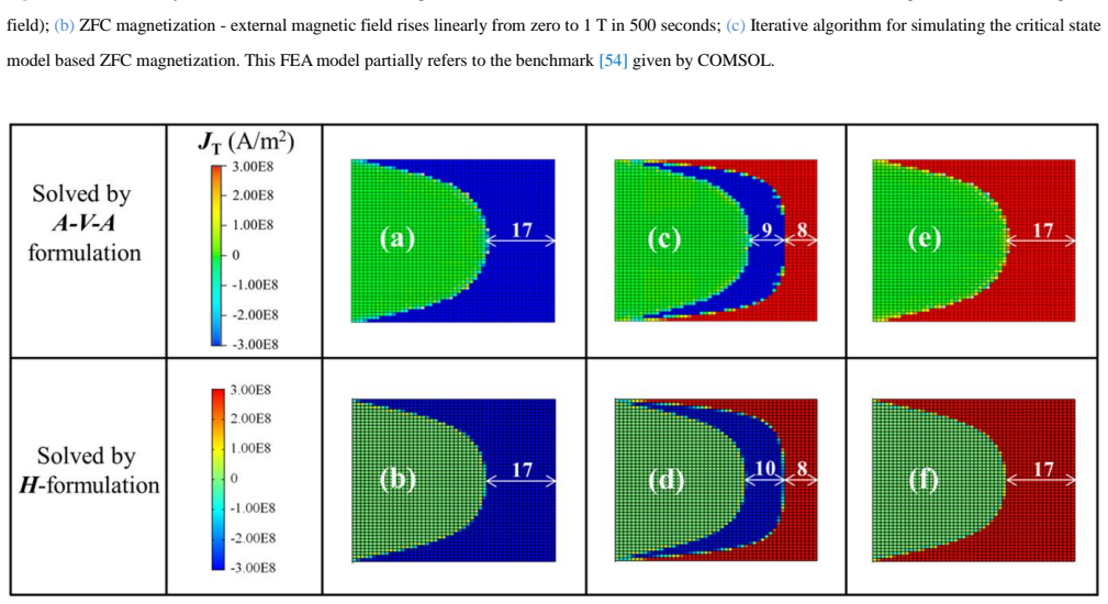
- [Sec. 2.1(c), 2.2; Eq. (5)] The critical-state ZFC result is in part manufactured by the algorithm rather than solved. After each load step, over-trapped elements are switched to ET-1 and their current is pinned to Jc (Section 2.1c), and at the end of the descending ramp the inner -Jc layer is explicitly forced by an additional BFE step (Section 2.2). Equation (5) is an ad hoc nodal-voltage condition introduced solely to keep that inner layer from decaying, with no derivation from Maxwell's equations or the Bean model. Please provide a derivation or a convergence argument showing that the forcing rule plus Eq. (5) reproduces the Bean critical state for general geometries and field histories; otherwise the only genuinely predictive quantity in the comparison with COMSOL is the location of the penetration front in a single axisymmetric disk.
- [Sec. 5.1.2 and 5.1.3; Fig. 16] The critical-state solutions are not independent of the numerical parameters ρ0 and T1. Figure 16(f) and (i) show that ρ0=10^-15 Ω·m or T1=5000 s produce a bulk that is 'not well penetrated at the ends,' and the text recommends re-assigning a smaller ρ0. For the Bean critical state, the final current distribution should be independent of these parameters, so the good agreement in Figure 2 is conditional on a hand-picked ρ0/T1 pair. Provide a selection criterion derived from the relevant time constants and demonstrate convergence to a parameter-independent solution (e.g., as ρ0 is reduced at fixed ramp time, or as the ramp time is shortened at fixed applied-field history).
- [Sec. 5.2.4; Fig. 17(j)-(l)] The flux-creep results depend strongly on the smoothing coefficient k1, which is not part of the E-J power law. k1=0.9 already produces 'abnormal penetrating elements,' and k1=0.8 or 0.7 yield inhomogeneous, nonconverged profiles. Since the paper claims easy convergence as an advantage, the method needs either a principled rule for choosing k1 (and by extension k2,k3) or a demonstration that the converged solution is independent of these coefficients over a suitable range.
- [Sec. 3; Figs. 6, 9, 10] All agreement claims with the COMSOL H-formulation are made visually or by counting penetrated elements in the mid-plane; no quantitative error measure is reported. Please add a quantitative comparison (for example the L2 or L∞ norm of the current-density difference over the bulk, or the trapped-field profile) and a convergence study with respect to load-step count and mesh size. Without such measures, 'agree well' remains unsubstantiated.
minor comments (7)
- [Fig. 8 caption] The caption of Figure 8(b) says 'flux creep model based ZFC magnetization,' but the section and figure describe FC magnetization; correct the label.
- [Fig. 9 caption] The Figure 9 caption lists panels (a), (c), (d), (e) while the text refers to (a)-(d); renumber the subfigures consistently.
- [Eq. (5)] Equation (5) should define V explicitly as the electric scalar potential and state the units of each quantity; the reader should not have to infer the meaning from context.
- [Secs. 2.1 and 3.1] The initial resistivity is given as ρ0=10^-16 Ω·m in Section 2.1 and ρ0=10^-17 Ω·m in Section 3.1; clarify whether this difference is intentional and how the value should be chosen in practice.
- [Figs. 2, 6, 9, 10] The current-density color maps have no visible color bars or labeled scales; add color bars and indicate the Jc value on each map.
- [Eq. (13)] The bracket and brace formatting in Eq. (13) appears garbled; typeset the strain-dependent Jc expression carefully.
- [Reference [53]] Reference [53] is incomplete: it lacks the year, volume, and page numbers; complete the citation.
Circularity Check
Critical-state agreement is partly built in: Jc is forced by BFE and the inner layer is inserted by hand; Jc(B)/Jc(ε) checks are tautological.
-
self definitional
[Section 2.2, ZFC field-descending algorithm (after load step N1+N2), Figure 2(c)]
"But the trapped JT in the inner layer is not exactly -3x10^8 A/m^2 even though we set the nodal voltage boundary at the beginning. A viable solution to approach the critical state model is to introduce an additional iterative step by using the “BFE” command to force the inner trapped JT to -3x10^8 A/m^2."
The critical-state model is implemented by imposing J=Jc in penetrated elements (Section 2.1c) and, after the field descent, by an extra BFE step that sets the inner layer to -3e8 A/m^2 by hand. The final ANSYS profile in Figure 2(c) is therefore manufactured to have the Bean-magnetization magnitudes, while COMSOL computes a physically relaxed inner layer (~-2.90e8 A/m^2). The comparison is between an imposed value and a computed one; only the penetration depth/front is a genuinely solved quantity. The nodal-voltage condition of Eq. (5) is likewise an invented ansatz whose stated role is to 'minimize the JT decay of the inner penetrated elements', not a derived Maxwell-equation result.
-
self definitional
[Section 4.2, Jc(B) implementation (Eq. 12, Kim model) and Figure 13]
"If |JT| for the ith bulk element is smaller than Jc but the ith bulk element has been penetrated before (mark = 1) we will use the “BFE” command to force the trapped JT to the updated Jc∙JT/|JT|. ... The relation between the trapped |JT| and B in each bulk element satisfies (12) seriously."
The IAM update rule sets every currently penetrated or previously penetrated element's current to the updated Jc(B) from Eq. (12) via the BFE command. Consequently the reported relation between trapped |JT| and local B is exactly the input Kim-model relation by construction; the statement that the result 'satisfies (12) seriously' is a restatement of the forcing rule, not an independent prediction. The same construction is used for the Jc(ε) case in Section 4.3.
1 more flagged steps
-
self definitional
[Section 4.3, Jc(ε) implementation (Eq. 13) and Figure 15]
"After the static mechanical analysis of load step-1 we extract the Von-Mises mechanical strain εeq of each bulk element, update the Jc according to (13) ... The relation between the trapped |JT| and εeq in each bulk element satisfies (13) seriously."
The algorithm updates Jc according to Eq. (13) and then forces penetrated or ever-penetrated elements to that updated value via BFE. The claimed agreement of the trapped-current map with Eq. (13) is therefore guaranteed by the update/forcing step itself; it does not independently test or predict the strain dependence of Jc.
full rationale
The central benchmark (Figures 2, 6, 9, 10) is an external COMSOL H-formulation calculation run by M. Ainslie using the same Jc, n, geometry, and field ramps; the IAM parameters (ρ0, k, N) are stability/tuning values, not fitted to COMSOL outputs. The core claim is therefore not a fitted-input-called-prediction, and the self-citations (refs 64 and 72) are used only for material properties and software openness, not as load-bearing derivation steps. However, the critical-state IAM is partially self-definitional: penetrated elements are switched to ET-1 and their current is pinned to Jc by the BFE command after every load step, and during ZFC descent the inner -Jc layer is explicitly inserted by an extra BFE step. The magnitude profile is thus imposed rather than solved, leaving the penetration front as the main genuinely predictive comparison with COMSOL. Sections 4.2 and 4.3 are more clearly circular: every previously penetrated element is forced, via BFE, to the updated Jc(B) or Jc(ε), so the assertions that the results 'satisfy (12)/(13) seriously' merely restate the forcing rules. Overall this is partial circularity, with independent content in the external benchmark and in the computed penetration fronts, but with several predicted profiles equivalent to their inputs by construction.
Assumptions & free parameters
free parameters (3)
- Initial resistivity rho0 of ReBCO elements =
10^-16 Ohm.m (critical state), 10^-17 Ohm.m (flux creep)
- Updating coefficients k1, k2, k3 =
k1=0.99 (ramp), k2=0.9 (hold), k3=0.99 (descend)
- Iterative load step counts N1, N2, N3 =
N1=200-1000; N2=200-500; N3=300-500
assumptions (6)
- standard math Quasi-static Maxwell equations in A-V/A form as solved by ANSYS Plane233 element.
- domain assumption Bean critical state model: |J|=Jc in penetrated regions, J=0 elsewhere.
- domain assumption E-J power law for flux creep: rho = (Ec/Jc)(|J|/Jc)^(n-1).
- domain assumption 2D axisymmetric approximation of the disk-shaped bulk.
- ad hoc to paper Forcing |J|=Jc in penetrated elements after each load step is a valid discrete representation of the critical state dynamics.
- ad hoc to paper The nodal voltage boundary condition V = -2*pi*r*rho0*Jc preserves the inner-layer trapped current without altering outer-layer penetration.
Cite this review
Pith. "Pith review of Magnetization Current Simulation of High Temperature Bulk Superconductors Using A-V-A Formulation and Iterative Algorithm Method: Critical State Model and Flux Creep Model." pith.science (2026). https://pith.science/paper/NUJCQ3E2
@misc{pith2026190804640,
  author       = {Pith},
  title        = {Pith review of: Magnetization Current Simulation of High Temperature Bulk Superconductors Using A-V-A Formulation and Iterative Algorithm Method: Critical State Model and Flux Creep Model},
  year         = {2026},
  howpublished = {\url{https://pith.science/paper/NUJCQ3E2}},
  note         = {Machine review of arXiv:1908.04640}
}
read the original abstract
In this work we will introduce the A-V-A formulation based iterative algorithm method (IAM) for simulating the magnetization current of high temperature superconductors. This new method embedded in ANSYS can simulate the critical state model by forcing the trapped current density to the critical current density Jc for all meshed superconducting elements after each iterative load step, as well as simulate the flux creep model by updating the E-J power law based resistivity values. The simulation results of a disk-shaped ReBCO bulk during zero field cooling (ZFC) or field cooling (FC) magnetization agree well with the simulation results from using the H-formulation in COMSOL. The computation time is shortened by using the A-V formulation in superconductor areas and the A-formulation in non-superconductor areas. This iterative method is further proved friendly for adding ferromagnetic materials into the FEA model or taking into account the magnetic field-dependent or mechanical strain-related critical current density of the superconductors. The influence factors for the magnetization simulation, including the specified iterative load steps, the initial resistivity, the ramping time and the updating coefficient, are discussed in detail. The A-V-A formulation based IAM, implemented in ANSYS, shows its unique advantages in adjustable computation time, multi-frame restart analysis and easy-convergence.
Figures

Figures from the paper (6 more)




Reference graph
Works this paper leans on
-
[1]
Introduction Magnetization current (screening current , shielding current or persistent current ) effect of commercial superconductors, usually un-desired, has been extensively studied in superconducting accelerator magnets [1-7], NMR magnets and high Tc superconducting coils [8-17] by using numerical simulation or experimental method . Recent studies sho...
work page 2020
-
[2]
The critical state model based iterative algorithm and its application in ZFC and FC magnetization 2.1. ZFC magnetization - external field rises from zero to 1 T Figure 1 (a) shows the 2D axis -symmetric half FEA model created in ANSYS for simulating the magnetization current in a disk -shaped ReBCO bulk (Φ25 mm, 10 mm thick) [54]. To app roach the superc...
work page 2020
-
[3]
The flux creep model based iterative algorithm and its application in ZFC and FC magnetization 3.1. ZFC magnetization - external field rises from zero to 1 T Different from the FEA model shown in Figure 1 (a), the ReBCO bulk (A-V formulation, ρ defined) and the non-superconductor areas (A-formulation, ρ undefined) are all meshed with the element type of P...
work page 2020
-
[4]
Implement B-H, Jc(B) and Jc(ε) into the magnetization process In this section the possibility of implementing B-H, Jc(B) and Jc(ε) into the magnetization process is investigated by “repeating” the simulation in Section-2.1. 4.1. Trapped JT in ReBCO bulk when including ferromagnetic materials Simulation or experimental studies show that ferromagnetic mater...
work page 2020
-
[5]
Discussion To further understand the mechanism behind the A-V-A formulation based IAM we repeat the simulation case shown in Section-2.1 (critical state model, Jc=3x10⁸ A/m2) and the simulation case in Section-3.1 (flux creep model , Jc=3x10⁸ A/m2, n=20) by defining varied load steps (N1), initial resistivity (ρ0), ramping time (T1) and updating coefficie...
work page 2020
-
[6]
Conclusion A series of magnetization simulation s on disk-shaped ReBCO bulk are carried out by implementing the A-V-A formulation based iterative algorithm method into ANSYS. This new method is proved feasible to simulate the ReBCO bulk ’s magnetization current during ZFC or FC magnetization for both critical state model and flux creep model. It is also p...
work page 1997
Reviewed August 14, 2026 · model on record in the stance chip above.
Discussion (0). Continue with ORCID to comment.