REVIEW 2 major objections 5 minor 1 cited by
Any valid lower confidence bound ordered by a statistic T is at most as large as the solution of a single optimization problem, which can be relaxed to a linear-size MILP.
Reviewed by Pith at T0; open to challenge. T0 means a machine referee read the full paper against a public rubric. the ladder, T0–T4 →
T0 review · grok-4.5
2026-07-14 12:10 UTC pith:O6DYJWLM
load-bearing objection Clean reduction of T-ordered mean LCBs to an optimization problem plus a usable linear-size MILP lower bound; the sample-approximation tightness gap is real but does not break validity. the 2 major comments →
Towards Automated Confidence Bound Provers and Searchers
The pith
A machine-rendered reading of the paper's core claim, the machinery that carries it, and where it could break.
Core claim
For any set of distributions F and any statistic T, the optimization problem that returns the greatest lower bound on a parameter theta among all F that still assign probability greater than alpha to the event T(X) greater than or equal to T(x) is itself a valid (1-alpha) lower confidence bound; moreover it dominates every other valid bound that is ordered by the same T.
What carries the argument
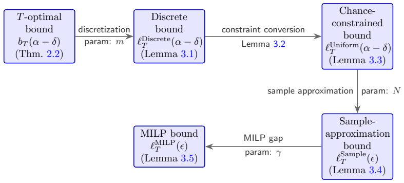
The T-order optimal bound b^F_T, defined by that optimization problem, together with its linear-size mixed-integer linear programming relaxation obtained by discretization, conversion to a chance constraint, and sample-average approximation.
Load-bearing premise
The sample-average approximation of the chance constraint is only guaranteed to stay below the true optimum with high probability under a conservative sample-size formula; the paper leaves open whether the approximation becomes arbitrarily tight as more samples are taken.
What would settle it
Drive the discretization, sample-size and MIP-gap parameters to their theoretical limits for the sample-mean ordering and check whether the computed MILP value converges to the closed-form T-optimal expression given by Luczak et al. for small n; systematic under-shoot would falsify tightness of the overall pipeline.
If this is right
- Any existing valid bound ordered by T can be fed into the MILP and returned as a (weakly) tighter valid bound for the same ordering.
- Any unproven ordering T can be turned into a proven valid bound simply by solving the corresponding MILP.
- Proving a candidate formula f is valid reduces to verifying that f(x) never exceeds the MILP value for every x.
- An automated searcher can optimize over order functions T while remaining inside the class of valid bounds.
- When the true support is a proper subset of [0,1], the same MILP automatically incorporates the extra information and can produce strictly tighter numbers than classical bounds that ignore it.
Where Pith is reading between the lines
- The same optimization-plus-MILP template could be reused for other parameters such as quantiles or for upper confidence bounds by a trivial sign flip.
- Once a library of pre-computed MILP tables indexed by T(x) exists, real-time application of the new bounds becomes as cheap as evaluating Hoeffding's formula.
- The open tightness question for the sample-average step is the single bottleneck that, if closed, would turn the method into a fully automated prover capable of recovering classical closed-form bounds as special cases.
Editorial analysis
A structured set of objections, weighed in public.
Referee Report
Summary. The paper formulates the tightest (1-α) lower confidence bound ordered by a statistic T as the optimization problem b^F_T(x,α) = inf { heta(F) : F∈F, P_F(T(X)≥T(x))>α} (Definition 2.1). Theorem 2.1 proves validity via the probability-integral transform; Theorem 2.2 proves that every valid T-ordered LCB is dominated by b^F_T. For F = all distributions on [0,1] and monotonic T the authors discretize the support (Lemma 3.1), convert the tail constraint into a chance constraint (Lemma 3.2–3.3), replace the chance constraint by a sample-average approximation (Lemma 3.4), and encode the resulting program as a linear-size MILP (Lemma 3.5). Theorem 3.1 assembles these steps into a high-probability validity guarantee for the MILP lower bound ℓ^MILP_T. Small-scale experiments (n=3 and n=10) illustrate the construction for the sample mean, Anderson’s bound and an approximate Gaffke bound.
Significance. If the reduction is correct, the work supplies a systematic, optimizable route from an arbitrary order function T to a valid LCB that is at least as tight as any previously known T-ordered bound. The optimality theorem (2.2) and the linear-size MILP encoding for linear monotonic T are concrete technical contributions that could automate bound tuning, conversion and (with further work) automated proving. The paper is explicit about remaining gaps (sample-approximation tightness, non-monotonic T, unbounded support) and therefore does not over-claim. The machine-readable MILP formulation and the clear separation of free parameters (m,N,ε,γ,M) are strengths that make the result reproducible and extensible.
major comments (2)
- Section 3.5 and the caption of Figure 1 explicitly leave open whether the sample-average approximation ℓ^Sample can be driven arbitrarily close to the chance-constrained value ℓ^Uniform as N o∞. Consequently Theorem 3.1 only certifies that ℓ^MILP is a valid (1-α) LCB; it does not certify that ℓ^MILP can be made arbitrarily close to the true T-optimal bound b^F_T even after m earrow and γ earrow0. The abstract and the “Automated Bound Tuning” claim in §1.2 therefore over-state what is currently proved. Either a convergence argument for the SAA (or a citation to a suitable existing result) or a clear restriction of the claims to “valid lower bounds that improve on T for some samples” is required.
- The experimental section (§4) uses N=100, M=10, m=50 and reports large standard deviations across the 10 independent runs (Figure 2). With these parameters the MILP bound is often only marginally better than the order function itself and the Monte-Carlo variability is comparable to the reported improvement. The paper needs either substantially larger N (or a tighter concentration inequality) that demonstrably reduces the variance, or an explicit statement that the current numbers are only a proof-of-concept and do not yet establish practical superiority.
minor comments (5)
- Notation for the ordered sample (X_{(i)}, x_{(i)}) is introduced late and then used inconsistently with the vector notation x⪡y; a short notational paragraph early in §2 would help.
- The MIP-gap analysis in Lemma 3.5 assumes the solver maximises 1- heta; the statement should also cover the direct minimisation of heta that appears in the algorithm box of Appendix A.
- Figure 1 caption claims that decreasing γ and increasing m make ℓ^MILP arbitrarily close to its targets; the claim is true only for the discretisation and MIP-gap steps, not for the SAA step that is left open.
- Several footnotes credit Gemini for code and proof fragments; a single acknowledgement sentence would be cleaner and more conventional.
- The phrase “linear-size mixed-integer linear program” appears in the abstract and introduction; the precise dependence on n,m,N should be stated once (O(N n m) binary variables) so that readers can judge scalability.
Circularity Check
No circularity: optimality of b^F_T and validity of the MILP lower bound are derived from the definition of a valid LCB plus standard probability tools, without self-referential fits or load-bearing self-citations.
full rationale
The central claim (Theorem 2.2) states that any valid T-ordered LCB g satisfies g(x) ≤ b^F_T(x,α) for every x, where b^F_T is defined by the optimization problem in Definition 2.1. The proof proceeds by contradiction from that definition together with the probability-integral-transform bound (Lemma C.1) and does not presuppose the conclusion. Validity of b itself (Theorem 2.1) likewise follows directly from the same PIT argument. The subsequent discretization (Lemma 3.1), conversion to chance constraints (Lemma 3.2), sample-average approximation (Lemmas 3.4/C.4–C.6) and MILP encoding (Lemma 3.5) are standard, one-directional relaxations that preserve the lower-bound property under the stated monotonicity assumption on T; none of them re-introduces the target quantity as an input. Prior work by the same authors (Phan et al. 2021) is cited only for Anderson coefficients used in experiments and for comparison; it is never invoked as a uniqueness theorem or as a premise that forces the new optimality claim. No free parameters are fitted to the quantity being proved. The only acknowledged gap (sample approximation may remain strictly loose as N o∞) is an incompleteness of tightness, not a circular reduction. Consequently the derivation chain is self-contained and non-circular.
Axiom & Free-Parameter Ledger
free parameters (3)
- discretization size m
- sample-approximation size N and significance ε
- MIP gap γ and number of independent runs M
axioms (5)
- standard math Probability integral transform: for any continuous CDF F, P(F(X) ≤ y) ≤ y
- domain assumption If F first-order stochastically dominates G then heta(F) ≥ heta(G) for the mean (and more generally for parameters monotone under stochastic dominance)
- domain assumption T is monotonic: y ≼ z implies T(y) ≤ T(z)
- domain assumption Support of every F ∈ F is contained in [0,1]
- standard math Hoeffding’s inequality supplies a sufficient sample size N for the sample-average approximation of a chance constraint
invented entities (3)
-
T-optimal bound b^F_T
no independent evidence
-
order function T
no independent evidence
-
MILP lower bound ℓ^MILP_T
no independent evidence
read the original abstract
In this work we lay the groundwork for automating the process of finding and proving the validity of lower confidence bounds of the mean. Our key finding is based on the observation that finding an optimal confidence bound under certain conditions can be formulated as an optimization problem. We use this observation to show that any valid confidence bound (such as Hoeffding's) must be a relaxation of a certain optimization problem. To automatically find and prove confidence bounds, we need to automate the process of defining and finding such a relaxation. We define a family of relaxations parameterized by a function called the order function. This family of relaxations can approximate any other target relaxation such as Hoeffding's by using the target as the order function. When the order function is linear (such as the sample mean in the case of Hoeffding's), our relaxation is a linear-size mixed-integer linear program.
Figures

Forward citations
Cited by 1 Pith paper
-
On the Order-Conditional Optimality of Gaffke's Bound
Gaffke's bound is Buehler-optimal within the class of lower confidence bounds that induce its own sample ordering, for the maximum marginal mean of independent nonnegative variables.
Reference graph
Works this paper leans on
-
[1]
doi: 10.1007/978-1-4939-1384-8 8. URLhttps://link.springer.com/chapter/10. 1007/978-1-4939-1384-8_8. Erik Learned-Miller. On the admissibility of bounds on the mean of discrete, scalar probability distributions from an iid sample.arXiv preprint arXiv:2502.17223, 2025. Erik Learned-Miller and Philip S. Thomas. A new confidence interval for the mean of a bo...
work page internal anchor Pith review Pith/arXiv arXiv doi:10.1007/978-1-4939-1384-8 2025
-
[2]
The meaning of the parameters are noted below: •δis to account for the probability that the sample approximation solution is not a lower bound of the chance-constrained program
Inputs: Sample sizen, samplex∈R n, monotonic functionT:R n →R, thresholdsα, ϵ, δ such that 0< α <1,0< δ < α,0< ϵ≤α−δ, MIP gapγ≥0, natural positive numbers m, N∈N, m, N≥1. The meaning of the parameters are noted below: •δis to account for the probability that the sample approximation solution is not a lower bound of the chance-constrained program. To accou...
-
[3]
For eachi,1≤i≤N: •Sampleni.i.d uniform random variablesU i ∈(0,1] n •SortU i in non-increasing order so that∀j,1≤j≤n−1 :U i j ≥U i j+1
Letv k := k m. For eachi,1≤i≤N: •Sampleni.i.d uniform random variablesU i ∈(0,1] n •SortU i in non-increasing order so that∀j,1≤j≤n−1 :U i j ≥U i j+1
-
[4]
(62) This is a MILP except for the objectiveθ(H v⊕1,f ) and the constraintT(y i)≥T(x) where T(x) is a constant
Solve the followingMMILPs within MIP gapγwithT, ϵ, m, N,U, Mchosen from previous steps: uMILP T (x, ϵ, m, N,U, γ) = infθ(H v⊕1,f ) (52) such that: 0≤f 1 ≤ · · · ≤f m = 1 (53) ∀i,1≤i≤N:z i ∈ {0,1}(54) ∀i, j, k,1≤i≤N,1≤j≤n,1≤k≤m:w i,j,k ∈ {0,1}(55) ∀i, j, k,1≤i≤N,1≤j≤n,1≤k≤m:w i,j,k ≤w i,j,k+1 (56) ∀i, j, k,1≤i≤N,1≤j≤n,1≤k≤m:w i,j,k ≥w i,j+1,k (57) NX i=1 z...
-
[5]
Setℓ MILP :=u−∆ m to be the output valid lower bound
Letube the lower bound of the objective that the MILP solver output. Setℓ MILP :=u−∆ m to be the output valid lower bound. In the case whenθis the mean, for implementation convenience, we maximize 1−θinstead of minimizingθ. Letrbe the upper bound of the objective 1−θthat the MILP solver output. Letu:= 1−r. Setℓ MILP :=u−∆ m to be the output valid lower bo...
2021
-
[6]
The output of the MILP is a valid bound for any value ofN ′ ≥1, but the largerN ′ is, the output will be more likely be better than Gaffke’s bound
ChooseN ′ to be number of samples to compute the random Gaffke’s bound. The output of the MILP is a valid bound for any value ofN ′ ≥1, but the largerN ′ is, the output will be more likely be better than Gaffke’s bound
-
[7]
•SortA i′ in non-decreasing order so that∀j,1≤j≤n−1 :A i′ j ≤A i′ j+1
For eachi ′,1≤i ′ ≤N ′: •Sampleni.i.d uniform random variablesA i′ ∈[0,1] n. •SortA i′ in non-decreasing order so that∀j,1≤j≤n−1 :A i′ j ≤A i′ j+1. Letadenote the sample value ofA. We sampleajust once at the beginning and useT a for all samplesx. The bound will be valid sinceT a is just a function. Define the functionT a(x) to be:
-
[8]
Computingm i′ :=µ(H (1−x)⊕1,ai′ ) for everyi ′
-
[9]
Sort theN ′ value computed in the previous step so thatm 1 ≤m 2 ≤ · · ·m N ′. 19
-
[10]
Let ˆQa(1−α,1−x) :=m q
Letq:=⌈N ′(1−α)⌉. Let ˆQa(1−α,1−x) :=m q
-
[11]
Then we perform the algorithm in Appendix A withT a(yi)≥z iTa(x)
OutputT a(x) = 1− ˆQa(1−α,1−x). Then we perform the algorithm in Appendix A withT a(yi)≥z iTa(x). The constraintT a(yi)≥ ziTa(x) is equivalent to 1−zi+zi ˆQa(1−α,1−x)≥ ˆQa(1−α,1−y i). Whenz i = 1, ˆQa(1−α,1−x)≥ ˆQa(1−α,1−y i) is equivalent to ˆQa(1−α,1−x)≥µ(H (1−yi)⊕1,ai′ ) for⌈N ′(1−α)⌉values ofi ′. Using the big M method for counting where ifc i,i′ = 1 ...
2021
-
[12]
Thereforeu T (x, m)≥b F T (x)
To computeu T (x, m) we are searching over a subset ofF. Thereforeu T (x, m)≥b F T (x)
-
[13]
We will now show thatb F T (x)≥ℓ Discrete T (x, m). For any CDFF∈ C, we will show thatF(v)∈ Vand the CDFH v⊕1,F(v) satisfies: θ(Hv⊕1,F(v) )−∆ m ≤θ(F).(114) •Since the support is lower bounded by 0, the CDFFfirst order stochastically dominates Hv⊕0,F(v) . Thereforeθ(F)≥θ(H v⊕0,F(v) ). We have: θ(Hv⊕1,F(v) )−θ(F)≤θ(H v⊕1,F(v) )−θ(H v⊕0,F(v) ) (115) ≤∆ m.(11...
-
[14]
The gap between the upper boundu Discrete T (x, m) and the lower boundℓ Discrete T (x, m) can be bounded by ∆ m
It remains to show thatu Discrete T (x, m)−b F T (x)≤∆ m andb F T (x)−ℓ Discrete T (x, m)≤∆ m. The gap between the upper boundu Discrete T (x, m) and the lower boundℓ Discrete T (x, m) can be bounded by ∆ m. Therefore the gap betweenb F T (x) and the upper bound (or the lower bound) is at most ∆ m. C.3.2 Proofs of Section 3.2 Now we will prove Lemma 3.2 a...
2021
discussion (0)
Sign in with ORCID, Apple, or X to comment. Anyone can read and Pith papers without signing in.