REVIEW 2 major objections 6 minor 35 references
Individual Treatment Effect: Prediction Intervals and Sharp Bounds
T0 review · 2 major / 6 minor · reviewed 2026-08-07 · deepseek-v4-flash
Pith's one-line read The paper proves that in large randomized experiments the individual treatment effect is only partially identified, and characterizes exactly which prediction intervals can be guaranteed and how sharply the ITE distribution can be bounded…
desk verdict A genuinely useful binary-outcome taxonomy plus a plausible sharp pmf bound whose upper-bound proof has a real indexing error, so the central new claim is unproven as printed. read the letter →
The pith
A machine-rendered reading of the paper's core claim, the machinery that carries it, and where it could break.
The reading
What carries the argument
The carrying object is the collection of all couplings of the two potential-outcome marginals $P(Y_1)$ and $P(Y_0)$, the only part of the joint distribution identified under randomization. The proofs use Fr\'echet cell bounds on individual joint probabilities $P(Y_1=i,Y_0=j)$, sum these cell-wise bounds to bound $P(Y_1-Y_0=\delta)$, and then use Strassen's theorem for finite sets to construct joint distributions that attain the summed lower and upper bounds. In the binary setting, all couplings are parameterized by a single variable $t=P(Y_0=1,Y_1=1)$, which makes the six possible prediction intervals easy to check.
What would settle it
Take any two discrete marginal distributions and solve the linear program over the joint probability table to minimize and maximize $\sum_i P(Y_1=i,Y_0=i-\delta)$ subject to the marginals; if the optimum falls outside the interval in Equation (5), the sharpness claim fails. In the binary case, one can similarly enumerate $t\in[\max\{0,p+q-1\},\min\{p,q\}]$ and check whether any of the six candidate intervals has coverage at least $1-\alpha$ whenever $p$ and $q$ both lie between $\alpha$ and $1-\alpha$.
Extended reading notes
Core claim
The central discovery is that with only the marginal outcome distributions identified from a randomized experiment, the ITE inference problem reduces to a coupling problem, and sharp answers are available. For discrete potential outcomes with fixed marginals, the sharp bounds on $P(Y_1-Y_0=\delta)$ are $$\left[\sum_i \max\{P(Y_1=i)+P(Y_0=i-\delta)-1,0\},\;\sum_i \min\{P(Y_1=i),P(Y_0=i-\delta)\}\right],$$ with both endpoints attainable by some joint distribution compatible with the marginals. In the binary case, the paper gives a complete characterization: the only valid prediction intervals can be trivial, a singleton, or one of the two unit-length intervals, depending on the two response probabilities, and when both response probabilities are in $(\alpha,1-\alpha)$ the only valid interval is $[-1,1]$. The paper also shows that the Fisher null and the Neyman null can appear to conflict: a prediction interval of $\{0\}$ can be valid even when the average treatment effect is nonzero and its confidence interval excludes zero.
Load-bearing premise
The joint distribution of the potential outcomes is assumed completely unspecified beyond its marginals, and the large-sample analysis treats those marginals as exactly known.
Editorial extensions
If this is right
- In the binary-outcome case, if both response probabilities lie in $(\alpha,1-\alpha)$, the only valid $(1-\alpha)$ prediction interval is $[-1,1]$, so the trial data alone carry no nontrivial information about the individual treatment effect.
- The singleton $\{0\}$ is a valid prediction interval exactly when the sum of the two less-common observed outcome probabilities is at most $\alpha$; this can happen even when the average treatment effect is nonzero, so Fisher and Neyman nulls can appear to disagree.
- For continuous outcomes, any valid prediction interval must include the quantile-difference points $R'_1-L'_0$ and $L'_1-R'_0$, and the union-bound interval $[L_1-R_0,R_1-L_0]$ is always valid.
- The sharp pmf bounds of Theorem 12 apply to any discrete potential outcomes, including ordinal outcomes, so marginal data alone identify an exact range for $P(ITE=\delta)$ even though the ITE itself is not identified.
Reading between the lines
- The sum-of-Fr\'echet-bounds formula is a general fact about the difference or sum of two discrete random variables with fixed marginals, so it can be reused outside causal inference whenever only marginal distributions are known.
- In any realistic finite sample the marginals are estimated, so strictly valid finite-sample prediction intervals require accounting for estimation error; the large-sample results here set a lower envelope, not a plug-in recipe.
- The results clarify what data would be needed to escape the trivial interval: any information about dependence between $Y_0$ and $Y_1$, such as a cross-over design or a rank-preserving assumption, since marginal data alone cannot provide it.
- They also support a substantive policy point: aggregate evidence of a nonzero average effect does not imply that individualized treatment rules have detectable individual-level benefits, so decisions need to weigh external assumptions about effect heterogeneity.
Editorial analysis
A structured set of objections, weighed in public.
Referee Report
Summary. The paper studies what can be learned about individual treatment effects (ITE) from a large randomized experiment when only the marginal distributions of the potential outcomes are identified. In the binary outcome model it characterizes the valid (1−α) prediction intervals for the ITE as a function of the two response probabilities, including conditions for a trivial interval, singleton intervals, and non-negative/non-positive intervals. For continuous and ordinal outcomes it derives conservative intervals, points that must be included in any valid interval, and conditions under which zero must be included, using the sharp cdf bounds of Fan–Park and Zhang–Richardson. Its main new result is Theorem 12, which claims sharp bounds on the pmf of the ITE for discrete outcomes: P(Y1−Y0=δ) is bounded by the sum of per-cell Fréchet bounds. The paper concludes with a discussion contrasting ATE confidence intervals with ITE prediction intervals and a synthetic example where the ATE is nonzero while {0} is the only valid 95% prediction interval.
Significance. The results are useful and mostly correct. The binary-outcome characterization is clean and parameter-free: it depends only on the two marginal response probabilities and the nominal level, and it makes the distinction between Fisher and Neyman nulls concrete. Theorem 12, if established, is a valuable contribution because it gives an extremely simple sharp bound on the ITE pmf from marginals alone, extending earlier cdf bounds. The proof strategy is appropriate: the lower bound uses Strassen's theorem, and the upper bound attempts an explicit coupling construction. There are no fitted parameters, and the sharp bounds are checked against external Fréchet/Strassen benchmarks. However, the upper-bound half of Theorem 12 is not proven as printed, and a second rigor issue appears in the quantile definitions of Section 3.2; these need repair before the paper can be accepted.
major comments (2)
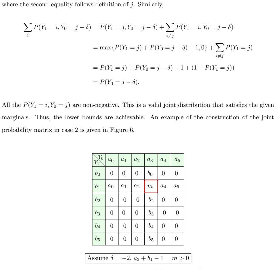
- [Section 5.1, Theorem 12, Eq. (5)] The upper-bound sharpness construction is invalid as printed. The set J2 is defined over columns j (with U_{j+δ}=P(Y0=j)), but the residual row factor subtracts I((i+δ)∈J2)P(Y0=i+δ); a J2-filled cell in row i lies at column i−δ, so the correct indicator is I(i−δ∈J2) and the correct subtracted mass is P(Y0=i−δ). The column factor has the symmetric error: I(j−δ∈J1)P(Y1=j−δ) should be I(j+δ∈J1)P(Y1=j+δ). The denominator s=1−∑_{J1}P(Y1=i)−∑_{J2}P(Y0=j) double-counts tied cells in which U_i=P(Y1=i)=P(Y0=i−δ); in such cases s is too small by the tied mass and can be zero or negative even when an (N1−n1)×(N2−n2) submatrix remains. Concretely, with p=(0.2,0.3,0.5), q=(0.5,0.3,0.2), δ=1, the printed row factor for i=0 equals 0.2−0.3<0. Since this construction is the only argument for sharpness of the upper bound, Theorem 12 is not proven as printed; the statement itself appears correct, and a residual-marginal argument (fill the diagonal cells with U_i, then complete the remaining transportation problem) would repair the proof.
- [Section 3.2] The 'must include' claim is not precisely stated. The quantities R'_0 and R'_1 are defined as maxima of sets of the form {ℓ:P(Y0>ℓ)>α}, which need not have a maximum; for a two-point distribution with P(Y0=0)=0.6, P(Y0=1)=0.4 and α=0.3, the set {ℓ:P(Y0>ℓ)>α} is (−∞,1), so R'_0 would be undefined. The intended objects are suprema (or quantiles defined with ≤/≥), and the proof's assertion that the minimum of the two tail probabilities is 'greater than α' is not true in general. The claim is plausibly correct after replacing the definitions, but as written it is not a theorem.
minor comments (6)
- [Table 1 / Section 4] The paper switches between p=P(Y=0|D=0), q=P(Y=0|D=1) in Section 4 and the response probabilities P(Y=1|D=j) used in Section 2 and Appendix A; because the two are complementary, the pmf formulas in Section 4 are easy to misread. It would help to state the convention explicitly once.
- [Section 3.1, proof of Eq. (1)] The final displayed inequality in the proof is written as P((Y1−Y0)∈[L1,R1])≥1−α, but it should be P((Y1−Y0)∈[L1−R0,R1−L0])≥1−α.
- [Proposition 14] The proof of Proposition 14 starts the contradiction with 'i≠j, k≠l'; the intended assumption should be i≠k and j≠l, matching the statement that at most one lower bound is nonzero when the row and column indices are both distinct.
- [Section 5.1, Case 2] The sentence 'Let P(Y1=i,Y0=k)=0 for any i≠j or k≠j−δ' should read 'i≠j and k≠j−δ' (or equivalently, all cells outside row j and column j−δ); as written the sentence contradicts the construction that follows.
- [Figure 7] Figure 7 is difficult to interpret: the permuted row and column labels do not clearly implement the definitions of J1 and J2, and the caption does not state which entries are the filled U_i cells; the figure should be redrawn after the proof is repaired.
- [Section 6.1] The synthetic example concludes a 95% prediction interval from estimated marginals; because the formal results require the true marginal distributions, the example should acknowledge that the conclusion is approximate or use a finite-sample construction.
Circularity Check
No significant circularity: the central bounds and interval characterizations follow from Fréchet/Strassen arguments and are not fitted to the target; the one self-citation (Zhang–Richardson 2024) is parameter-free and not load-bearing for Theorem 12.
full rationale
The paper's central claims are not circular. Theorem 12 bounds P(Y1−Y0=δ) by summing Fréchet cell bounds, but the paper addresses sharpness through Strassen's theorem (Koperberg 2024, external) for the lower bound and an explicit coupling construction for the upper bound; no parameter is fitted to the target probability, and the sharpness claim is not assumed from the bound itself. The binary-outcome characterization in Section 2 is derived from the one-parameter type parametrization together with Fréchet inequalities; conditions such as the trivial-interval characterization follow from direct extremal analysis of t, not from a self-citation. The only self-citation is Zhang and Richardson (2024), used for sharp cdf bounds in Section 3.3 and Appendix C. Those bounds are parameter-free, their stated assumptions are only the marginals of Y0 and Y1, and the paper's main pmf theorem (Theorem 12) does not depend on them, so the citation is independent support rather than a load-bearing loop. The supplied critique that the upper-bound construction in Theorem 12 has misindexed residual marginals and an ill-defined denominator s is a proof-rigor concern, not a circularity: it does not make the theorem's statement equivalent to its inputs by construction, and thus does not raise the circularity score.
Assumptions & free parameters
assumptions (5)
- domain assumption Randomization and consistency in a large RCT identify the marginal distributions of Y0 and Y1: P(Y=i|D=j)=P(Y^j=i).
- domain assumption The joint distribution of potential outcomes is unrestricted apart from these marginals; any coupling is possible.
- standard math Fréchet inequality bounds and Strassen's theorem for finite sets are valid.
- domain assumption Alpha is sufficiently bounded away from 0.5.
- domain assumption SUTVA and no interference hold in the covariate extension.
Cite this review
Pith. "Pith review of Individual Treatment Effect: Prediction Intervals and Sharp Bounds." pith.science (2026). https://pith.science/paper/OBQIYVYH
@misc{pith2026250607469,
  author       = {Pith},
  title        = {Pith review of: Individual Treatment Effect: Prediction Intervals and Sharp Bounds},
  year         = {2026},
  howpublished = {\url{https://pith.science/paper/OBQIYVYH}},
  note         = {Machine review of arXiv:2506.07469}
}
read the original abstract
Individual treatment effect (ITE) is often regarded as the ideal target of inference in causal analyses and has been the focus of several recent studies. In this paper, we describe the intrinsic limits regarding what can be learned concerning ITEs given data from large randomized experiments. We consider when a valid prediction interval for the ITE is informative and when it can be bounded away from zero. The joint distribution over potential outcomes is only partially identified from a randomized trial. Consequently, to be valid, an ITE prediction interval must be valid for all joint distribution consistent with the observed data and hence will in general be wider than that resulting from knowledge of this joint distribution. We characterize prediction intervals in the binary treatment and outcome setting, and extend these insights to models with continuous and ordinal outcomes. We derive sharp bounds on the probability mass function (pmf) of the individual treatment effect (ITE). Finally, we contrast prediction intervals for the ITE and confidence intervals for the average treatment effect (ATE). This also leads to the consideration of Fisher versus Neyman null hypotheses. While confidence intervals for the ATE shrink with increasing sample size due to its status as a population parameter, prediction intervals for the ITE generally do not vanish, leading to scenarios where one may reject the Neyman null yet still find evidence consistent with the Fisher null, highlighting the challenges of individualized decision-making under partial identification.
Figures


Figures from the paper (4 more)



Reference graph
Works this paper leans on
-
[1]
Blaker, H. (2000). Confidence curves and improved exact confidence intervals for discrete distributions. Canadian Journal of Statistics , 28(4):783--798
work page 2000
-
[2]
Brennan, J., Lahaie, S., Javanmard, A., Doudchenko, N., and Pouget-Abadie, J. (2024). Causal bootstrap for general randomized designs. arXiv preprint arXiv:2410.21464
work page Pith review arXiv 2024
-
[3]
Chernozhukov, V., W \"u thrich, K., and Zhu, Y. (2023). Toward personalized inference on individual treatment effects. Proceedings of the National Academy of Sciences , 120(7):e2300458120
work page 2023
-
[4]
Chiba, Y. (2015). Exact tests for the weak causal null hypothesis on a binary outcome in randomized trials. Journal of Biometrics & Biostatistics , 6(244)
work page 2015
-
[5]
Copas, J. (1973). Randomization models for the matched and unmatched 2 2 tables. Biometrika , 60(3):467--476
work page 1973
-
[6]
Cui, Y. (2021). Individualized decision-making under partial identification: three perspectives, two optimality results, and one paradox. arXiv preprint arXiv:2110.10961
arXiv 2021
-
[7]
P., Musio, M., and Fienberg, S
Dawid, A. P., Musio, M., and Fienberg, S. E. (2016). From statistical evidence to evidence of causality
work page 2016
-
[8]
Dawid, A. P. and Senn, S. (2023). Personalised decision-making without counterfactuals. arXiv preprint arXiv:2301.11976
arXiv 2023
Show all 35 references
-
[9]
Duarte, G., Finkelstein, N., Knox, D., Mummolo, J., and Shpitser, I. (2024). An automated approach to causal inference in discrete settings. Journal of the American Statistical Association , 119(547):1778--1793
2024
-
[10]
and Park, S
Fan, Y. and Park, S. S. (2010). Sharp bounds on the distribution of treatment effects and their statistical inference. Econometric Theory , 26(3):931--951
2010
-
[11]
Fisher, R. A. (1936). Design of experiments. British Medical Journal , 1(3923):554
1936
-
[12]
J., Nelsen, R
Frank, M. J., Nelsen, R. B., and Schweizer, B. (1987). Best-possible bounds for the distribution of a sum---a problem of kolmogorov. Probability theory and related fields , 74(2):199--211
1987
-
[13]
J., Fang, E
Huang, E. J., Fang, E. X., Hanley, D. F., and Rosenblum, M. (2017). Inequality in treatment benefits: Can we determine if a new treatment benefits the many or the few? Biostatistics , 18(2):308--324
2017
-
[14]
and Menzel, K
Imbens, G. and Menzel, K. (2018). A causal bootstrap. Technical report, National Bureau of Economic Research
2018
-
[15]
Jin, Y., Ren, Z., and Cand \`e s, E. J. (2023). Sensitivity analysis of individual treatment effects: A robust conformal inference approach. Proceedings of the National Academy of Sciences , 120(6):e2214889120
2023
-
[16]
Kallus, N. (2022a). Treatment effect risk: Bounds and inference. arXiv preprint arXiv:2201.05893
2022 arXiv
-
[17]
Kallus, N. (2022b). What's the harm? sharp bounds on the fraction negatively affected by treatment. Advances in Neural Information Processing Systems , 35:15996--16009
2022
-
[18]
and Tian, J
Kawakami, Y. and Tian, J. (2025). Mediation analysis for probabilities of causation. In Proceedings of the AAAI Conference on Artificial Intelligence , volume 39, pages 26823--26832
2025
-
[19]
Koperberg, T. (2024). Couplings and matchings: Combinatorial notes on strassen’s theorem. Statistics & Probability Letters , 209:110089
2024
-
[20]
and Cand \`e s, E
Lei, L. and Cand \`e s, E. J. (2021). Conformal inference of counterfactuals and individual treatment effects. Journal of the Royal Statistical Society Series B: Statistical Methodology , 83(5):911--938
2021
-
[21]
Lu, J., Ding, P., and Dasgupta, T. (2018). Treatment effects on ordinal outcomes: Causal estimands and sharp bounds. Journal of Educational and Behavioral Statistics , 43(5):540--567
2018
-
[22]
Makarov, G. (1982). Estimates for the distribution function of a sum of two random variables when the marginal distributions are fixed. Theory of Probability & its Applications , 26(4):803--806
1982
-
[23]
Mueller, S., Li, A., and Pearl, J. (2021). Causes of effects: Learning individual responses from population data. arXiv preprint arXiv:2104.13730
2021 arXiv
-
[24]
and Pearl, J
Mueller, S. and Pearl, J. (2022). Personalized decision making--a conceptual introduction. arXiv preprint arXiv:2208.09558
2022 arXiv
-
[25]
Mullahy, J. (2018). Individual results may vary: Inequality-probability bounds for some health-outcome treatment effects. Journal of Health Economics , 61:151--162
2018
-
[26]
and Hudgens, M
Rigdon, J. and Hudgens, M. G. (2015). Randomization inference for treatment effects on a binary outcome. Statistics in medicine , 34(6):924--935
2015
-
[27]
and Greenland, S
Robins, J. and Greenland, S. (1989). The probability of causation under a stochastic model for individual risk. Biometrics , pages 1125--1138
1989
-
[28]
Robins, J. M. (1988). Confidence intervals for causal parameters. Statistics in medicine , 7(7):773--785
1988
-
[29]
R \"u schendorf, L. (1982). Random variables with maximum sums. Advances in Applied Probability , 14(3):623--632
1982
-
[30]
A., and Janzing, D
Sani, N., Mastakouri, A. A., and Janzing, D. (2023). Bounding probabilities of causation through the causal marginal problem. arXiv preprint arXiv:2304.02023
2023 arXiv
-
[31]
and Pearl, J
Tian, J. and Pearl, J. (2000). Probabilities of causation: Bounds and identification. Annals of Mathematics and Artificial Intelligence , 28(1-4):287--313
2000
-
[32]
and Qiao, X
Wang, B. and Qiao, X. (2025). Conformal inference of individual treatment effects using conditional density estimates. arXiv preprint arXiv:2501.14933
2025 arXiv
-
[33]
Williamson, R. C. and Downs, T. (1990). Probabilistic arithmetic. i. numerical methods for calculating convolutions and dependency bounds. International journal of approximate reasoning , 4(2):89--158
1990
-
[34]
Yin, M., Shi, C., Wang, Y., and Blei, D. M. (2022). Conformal sensitivity analysis for individual treatment effects. Journal of the American Statistical Association , pages 1--14
2022
-
[35]
and Richardson, T
Zhang, Z. and Richardson, T. S. (2024). Bounds on the distribution of a sum of two random variables: Revisiting a problem of kolmogorov with application to individual treatment effects. arXiv preprint arXiv:2405.08806
2024 arXiv
Reviewed August 7, 2026 · model on record in the stance chip above.
Discussion (0). Sign in to comment.