REVIEW 4 major objections 5 minor 29 references
Transfer learning for scalability of neural-network quantum states
T0 review · 4 major / 5 minor · reviewed 2026-08-14 · deepseek-v4-flash
Pith's one-line read Trained neural-network quantum states can be reused to jump-start ground-state searches on larger spin systems, reaching the target faster and more accurately than a random start when the transferred pattern matches the magnetic phase.
desk verdict Transfer learning with (k,p)-tilings is a genuinely useful new trick for scaling NQS, but the headline 'more effective than cold-start' needs a cold-start effectiveness baseline that the current figures don't show. read the letter →
The pith
A machine-rendered reading of the paper's core claim, the machinery that carries it, and where it could break.
The reading
What carries the argument
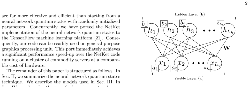
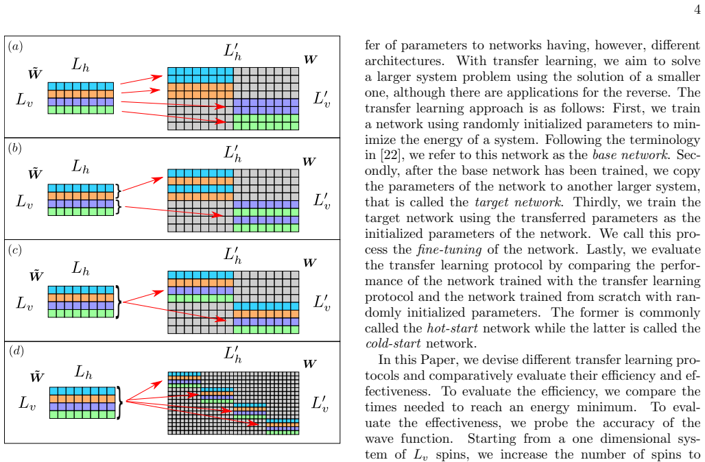
The central object is the restricted Boltzmann machine (RBM), a two-layer probabilistic neural network whose visible nodes encode spin configurations and whose squared amplitude defines the variational wave function. The transfer mechanism is the (k,p)-tiling rule: copy groups of k rows of the trained weight matrix and repeat each group p times across the target network's hidden nodes, filling the remaining weights with small random values. This mapping is what carries the learned correlations from the base system to the target; it succeeds only when the repeated tile matches the target phase's spin-spin correlation pattern. The implementation also ports the RBM energy minimization to GPU hardware, which is what makes the timing comparisons meaningful.
What would settle it
On the one-dimensional transverse-field Ising chain with $J_I = -2$ (antiferromagnetic phase), scale from 4 to 128 spins using the $(1,2)$-tiling, $(L,2)$-tiling, and a cold start with the paper's stopping criterion; the central claim fails if the $(L,2)$-tiling hot start does not reach the stopping criterion in less time and with lower mean relative energy error than the cold start over the 20 realizations.
Extended reading notes
Core claim
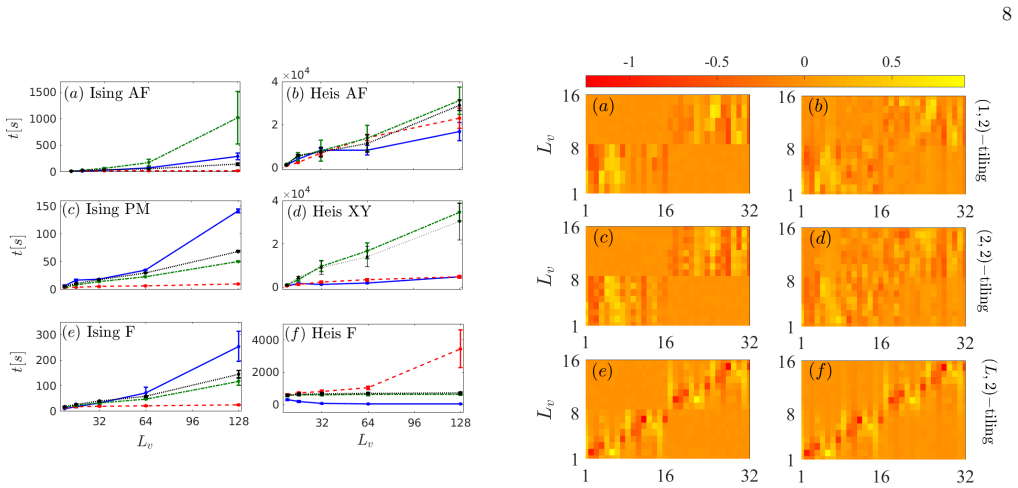
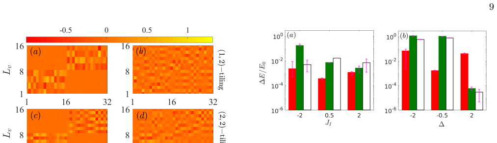
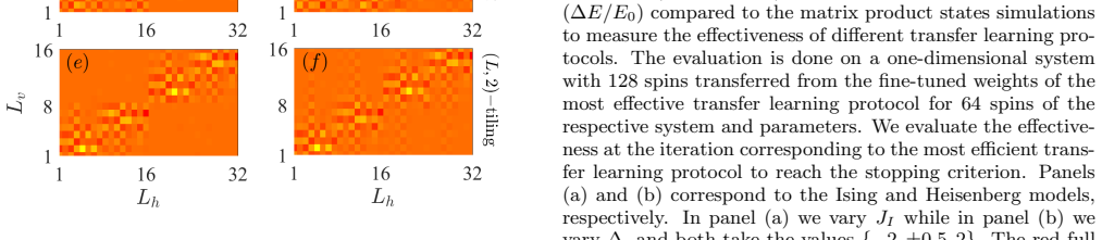
The paper's central claim is that transfer learning can improve the scalability of neural-network quantum states: a restricted Boltzmann machine trained on a small lattice can initialize the same ansatz on a larger lattice, and with the right tiling this hot start reaches the stopping criterion faster and with lower error than a cold start. The (L,2)-tiling protocol, which repeats the entire learned weight matrix in blocks, is the best all-around protocol for the one-dimensional transverse-field Ising model in all phases tested, and is competitive for the Heisenberg XXZ model in the antiferromagnetic and XY phases. The (1,2)- and (2,2)-tilings are better for the ferromagnetic Heisenberg phase, where magnetization is conserved, because they preserve the expected domain-wall structure. In the mismatched case, such as the (1,2)-tiling in the antiferromagnetic phase, the hot start can be slower and less accurate than a cold start, so the phase must be known in advance.
Load-bearing premise
The load-bearing assumption is that the target system's magnetic phase is known well enough to choose a tiling that preserves its correlation pattern; with a wrong phase choice, the transferred initialization is slower and less accurate than starting from random weights.
Editorial extensions
If this is right
- For one-dimensional transverse-field Ising chains, the (L,2)-tiling hot start reaches the stopping criterion faster and with lower mean relative energy error than a cold start in ferromagnetic, antiferromagnetic, and paramagnetic phases.
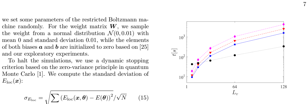
- For the Heisenberg XXZ chain at fixed zero magnetization, a cold start reaches the stopping criterion fastest but can be trapped in a local minimum, whereas the best phase-matched tiling gives lower energy error, except in the ferromagnetic phase where the (L,2)-tiling performs worse.
- Scaling a one-dimensional Ising chain from 4 to 128 spins in a single transfer already beats a cold start, and larger jumps early in the transfer followed by smaller jumps are generally better than uniform doubling.
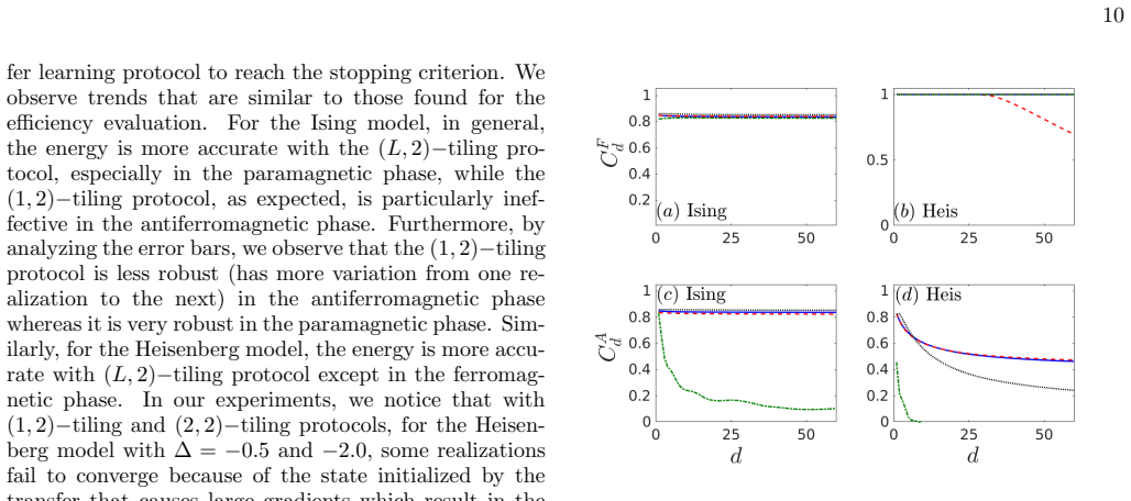
- The spin-spin correlators produced by the best phase-matched tiling track the matrix-product-state reference values more closely than mismatched tilings, so the accuracy gain is not limited to the energy.
- In the two-dimensional antiferromagnetic Heisenberg lattice, the (L,2)-tiling is the most efficient and effective of the three protocols tested.
Reading between the lines
- The phase-dependence of the best tiling suggests a practical selector that estimates the target's dominant correlations from a short cold start or a classical pre-solve and then chooses the matching tiling; the paper does not test such a selector.
- The same tiling idea should transfer between models that share a phase, for example from the antiferromagnetic Ising chain to the antiferromagnetic Heisenberg chain, because the correlation pattern the tiling preserves is the same; the paper lists cross-Hamiltonian transfer as future work rather than a result.
- For two-dimensional systems with striped or other non-uniform order, the isotropic (L,2)-tiling is only a special case; per-axis repetition factors could yield better performance, but this is not explored here.
- The reported non-convergent Heisenberg realizations after a bad transfer initialization imply that transfer learning changes the structure of the optimization landscape, so a transfer-distance diagnostic may need to be supplemented by a convergence-prediction criterion.
Signed reviews
Editorial analysis
A structured set of objections, weighed in public.
Referee Report
Summary. The manuscript proposes transfer learning protocols for restricted-Boltzmann-machine neural-network quantum states, in which weights trained for a small system are replicated (with prescribed (k,p)-tilings) to initialize a larger system. The protocols are benchmarked on the transverse-field Ising and Heisenberg XXZ models in one dimension and on the latter in two dimensions, with system sizes up to 128 and 8x8 spins and 20 realizations per setting. Efficiency is measured as time to a variance-based stopping criterion; effectiveness is measured by energy and spin-correlation errors relative to matrix-product-state or quantum Monte Carlo references. The paper reports that one protocol, (L,2)-tiling, is more efficient and effective than cold-start random initialization for the Ising model, that transfer protocols can avoid premature local minima for the Heisenberg model, and that a TensorFlow/GPU implementation is faster than the NetKet CPU implementation in comparable settings.
Significance. If the central claim is fully supported, this is a useful empirical contribution to scaling neural-network quantum states. The study is extensive in scope: two model families, multiple phases, 1D and 2D, several system sizes up to 128 and 8x8, 20 realizations, and external MPS/QMC references. The explicit transfer-distance diagnostic is a valuable idea, as is the physics-motivated distinction among tilings that preserve or destroy the relevant magnetic correlations. The TensorFlow port with GPU speedup is a practical contribution of independent interest. However, the headline claim of being 'far more effective and efficient' than cold-start is not currently backed by a direct cold-start effectiveness baseline in the main energy-error figures, and one figure excludes non-converged realizations without reporting exclusion counts. These gaps are fixable within the scope of the manuscript and do not, on the evidence presented, invalidate the underlying approach.
major comments (4)
- [§VI.B, Figs. 7 and 11] The abstract and conclusions claim that some transfer protocols are 'far more effective and efficient' than cold-start random initialization, and Sec. IV states that the evaluation will compare transfer-trained networks with networks trained from random initialization. The efficiency half of the claim is directly supported by Fig. 4, but the effectiveness half is not: Figs. 7 and 11(b) report energy errors of the transfer protocols only against MPS/QMC references, with no cold-start energy error plotted. The only quantitative cold-start effectiveness comparison is the 4-to-128 Ising scenario in Sec. VI.B and Fig. 10, where the transfer energy error is described as 30% better than cold-start. Please add cold-start energy-error baselines to the same effectiveness evaluations (at the same iteration counts used in Fig. 7), or explicitly restrict the claim to efficiency plus the specific scenarios where cold-start effectiveness has been measured.
- [§VI.B, Fig. 7(b)] The text states that for the Heisenberg model with Δ=-0.5 and Δ=-2.0, 'some realizations' of the (1,2)- and (2,2)-tiling protocols fail to converge because of large gradients, and that these extreme cases are not included in the error bars of Fig. 7(b). The number of excluded realizations is not reported for any protocol, phase, or size. Because these excluded runs belong to the very protocols against which (L,2)-tiling is compared, the reported error bars may systematically understate the failure rate and variance of those protocols. Please report the exclusion count for every affected entry and provide a sensitivity analysis, such as a conservative worst-case treatment of the non-converged realizations.
- [§VI.B, Fig. 7 and caption] The three transfer protocols are all initialized from the same base network, namely the solution of the 'most effective protocol' at Lv=64. This common-base choice is intended to make the comparison fair, but it may instead disadvantage the (1,2)- and (2,2)-tilings, whose weight-copying rules are designed to be applied to base weights produced by those same protocols. A base trained under (L,2)-tiling will have a weight structure that the (1,2)- and (2,2)-tilings may not preserve. Please either use each protocol's own base network at Lv=64 for the Lv=128 evaluation, or justify why a common base is the appropriate comparison and report the protocol that supplied the base for each panel.
- [§V.B and §VI.B, definition of effectiveness evaluation] The effectiveness results in Fig. 7 are evaluated at a fixed number of iterations determined by the stopping criterion of the fastest transfer protocol, not at each protocol's own stopping point. This makes the comparison a time-limited or iteration-limited accuracy comparison rather than a comparison of final converged states, which is how 'effectiveness' is defined in Sec. V. The paper should state this explicitly in the main text and in the figure captions, and should also include the cold-start protocol in the same fixed-iteration evaluation. Otherwise the reader cannot separate accuracy at equal computational budget from accuracy at convergence, which matters for the paper's claim that transfer learning improves scalability.
minor comments (5)
- [§V.A, Eqs. (12) and (13)] The correlators CF_d and CA_d are defined with a factor 1/(d-1), but the text and figures evaluate them for d starting at 1, for which the denominator vanishes. Please either start the range at d=2 or define the d=1 case separately.
- [§V.A, Eq. (14)] The index order in Eq. (14) is inconsistent with the convention W_ji used earlier in the paper: Eq. (14) writes W_{i,j}, while the surrounding text and Fig. 5 use W_{j,i}. Please make the indices consistent.
- [§II, Eqs. (7) and (8)] The text says that a hidden configuration is sampled from p(h|x) using Eq. (7) and that a visible configuration is sampled from p(h|x) using Eq. (8); the two formulas appear to be labeled in the opposite order. Please correct the labeling or the description.
- [§V.B] The parameters of the optimization are said to be determined from the literature or from a grid search, but no grid, range, or selection criterion is given. For reproducibility, please list the grid-search choices and the selected values.
- [§IV] The statement that simulations with biases set to zero and with variable biases yield very close results is not accompanied by data. Please show a comparison or provide a reference to a figure/table supporting this claim.
Circularity Check
No circularity: transfer protocols are benchmarked against external MPS/QMC references and cold-start baselines; no fitted input is renamed as a prediction.
full rationale
The paper is an empirical comparative study, not a derivation from fitted parameters. The transfer protocols are defined as explicit weight-mapping rules, the (k,p)-tiling constructions in Sec. IV, and their efficiency is measured as wall-clock time to a fixed stopping criterion against cold-start runs (Fig. 4, Fig. 10, Fig. 11a), while their effectiveness is measured as relative energy and correlation errors against independent external references: matrix product states for the one-dimensional models and quantum Monte Carlo for the two-dimensional Heisenberg model. The transfer distance D in Eq. (14) is a post hoc diagnostic of how much the weights change during fine-tuning; it is not a fitted parameter from which the reported energy errors are derived. The paper's central claim, that some transfer protocols are more effective and efficient than cold-start, is therefore not equivalent to its inputs by construction. The main caveats, such as the exclusion of some non-converged Heisenberg realizations from Fig. 7(b) and the requirement in Sec. VII that a tiling protocol adapted to the phase must be chosen, concern evidential support and applicability rather than circularity. No load-bearing self-citation is present; the cited methodological foundations, Carleo and Troyer and Yosinski et al., are external to the authors of this paper. Accordingly, no circular step can be exhibited.
Assumptions & free parameters
free parameters (4)
- Hidden density alpha (Lh/Lv) =
2
- Initial learning rate =
0.001
- Stopping threshold epsilon_sigma =
0.005
- Maximum epochs epsilon_epoch =
30000
assumptions (4)
- domain assumption The ground states of the considered spin models can be written with real nonnegative amplitudes in the chosen basis, so that a real RBM suffices.
- domain assumption A restricted Boltzmann machine with alpha=2 is expressive enough to approximate these ground states to the reported accuracy.
- ad hoc to paper Features learned by an RBM for a small system remain useful after (k,p)-tiling replication for a larger system.
- domain assumption The local-energy variance epsilon_sigma = 0.005 is a fair and comparable stopping criterion across protocols.
Cite this review
Pith. "Pith review of Transfer learning for scalability of neural-network quantum states." pith.science (2026). https://pith.science/paper/OSA4ZW6W
@misc{pith2026190809883,
  author       = {Pith},
  title        = {Pith review of: Transfer learning for scalability of neural-network quantum states},
  year         = {2026},
  howpublished = {\url{https://pith.science/paper/OSA4ZW6W}},
  note         = {Machine review of arXiv:1908.09883}
}
read the original abstract
Neural-network quantum states have shown great potential for the study of many-body quantum systems. In statistical machine learning, transfer learning designates protocols reusing features of a machine learning model trained for a problem to solve a possibly related but different problem. We propose to evaluate the potential of transfer learning to improve the scalability of neural-network quantum states. We devise and present physics-inspired transfer learning protocols, reusing the features of neural-network quantum states learned for the computation of the ground state of a small system for systems of larger sizes. We implement different protocols for restricted Boltzmann machines on general-purpose graphics processing units. This implementation alone yields a speedup over existing implementations on multi-core and distributed central processing units in comparable settings. We empirically and comparatively evaluate the efficiency (time) and effectiveness (accuracy) of different transfer learning protocols as we scale the system size in different models and different quantum phases. Namely, we consider both the transverse field Ising and Heisenberg XXZ models in one dimension, and also in two dimensions for the latter, with system sizes up to 128 and 8 x 8 spins. We empirically demonstrate that some of the transfer learning protocols that we have devised can be far more effective and efficient than starting from neural-network quantum states with randomly initialized parameters.
Figures
Figures from the paper (7 more)


Reference graph
Works this paper leans on
-
[1]
J. Gubernatis, N. Kawashima, and P. Werner, Quan- tum Monte Carlo Methods: Algorithms for Lattice Mod- els (Cambridge University Press, 2016)
work page 2016
-
[2]
A. W. Sandvik, Physical Review B 56, 11678 (1997)
work page 1997
-
[3]
Or´ us, Ann
R. Or´ us, Ann. Phys.349, 117 (2014)
2014
- [4]
-
[5]
Schollw¨ ock, Rev
U. Schollw¨ ock, Rev. Mod. Phys.77, 259 (2005)
2005
-
[6]
Schollw¨ ock, Ann
U. Schollw¨ ock, Ann. Phys.326, 96 (2011)
2011
-
[7]
S. R. White, Phys. Rev. Lett. 69, 2863 (1992)
1992
-
[8]
The blue empty bars are for cold-start, red full bars are for (L, 2)−tiling protocol, green full bars for (1, 2)−tiling pro- tocol, and black empty bars for (2 , 2)−tiling protocol. Panel (b) shows the effectiveness of different transfer learning pro- tocols in terms of the ground state energy. The panel shows the mean relative error of different transfer le...
Show all 29 references
-
[9]
Georges, G
A. Georges, G. Kotliar, W. Krauth, and M. J. Rozen- berg, Rev. Mod. Phys. 68, 13 (1996)
1996
-
[10]
Metzner and D
W. Metzner and D. Vollhardt, Phys. Rev. Lett. 62, 324 (1989)
1989
-
[11]
Georges and G
A. Georges and G. Kotliar, Phys. Rev. B 45, 6479 (1992)
1992
-
[12]
Carleo and M
G. Carleo and M. Troyer, Science 355, 602 (2017)
2017
-
[13]
K. Choo, G. Carleo, N. Regnault, and T. Neupert, Phys. Rev. Lett. 121, 167204 (2018)
2018
-
[14]
Czischek, M
S. Czischek, M. G¨ arttner, and T. Gasenzer, Phys. Rev. B 98, 024311 (2018)
2018
-
[15]
D.-L. Deng, X. Li, and S. D. Sarma, Phys. Rev. X 7, 021021 (2017)
2017
-
[16]
Melko, G
R. Melko, G. Carleo, J. Carrasquilla, and J. I. Cirac, Nature Physics (2019)
2019
-
[17]
Das Sarma, D.-L
S. Das Sarma, D.-L. Deng, and L.-M. Duan, Physics Today 72, 48 (2019)
2019
-
[18]
Carleo, J
G. Carleo, J. I. Cirac, K. Cranmer, L. Daudet, M. Schuld, N. Tishby, L. Vogt-Maranto, and L. Zdeborov´ a, arxiv:1903.10563 (2019)
2019 arXiv
-
[19]
K. Choo, T. Neupert, and G. Carleo, arxiv:1903.06713 (2019)
2019 arXiv
-
[20]
Carleo, K
G. Carleo, K. Choo, D. Hofmann, J. E. Smith, T. West- erhout, F. Alet, E. J. Davis, S. Efthymiou, I. Glasser, S.-H. Lin, et al., arXiv:1904.00031 (2019)
2019 arXiv
-
[21]
T. G. Dietterich, L. Pratt, and S. Thrun, Mach. Learn. 28 (1997)
1997
-
[22]
Abadi, P
M. Abadi, P. Barham, J. Chen, Z. Chen, A. Davis, J. Dean, M. Devin, S. Ghemawat, G. Irving, M. Isard, et al., in OSDI, Vol. 16 (2016) pp. 265–283
2016
-
[23]
Yosinski, J
J. Yosinski, J. Clune, Y. Bengio, and H. Lipson, in Ad- vances in neural information processing systems (2014) pp. 3320–3328
2014
-
[24]
Neural net- works for machine learning lecture 6a overview of mini– batch gradient descent,
G. Hinton, N. Srivastava, and K. Swersky, “Neural net- works for machine learning lecture 6a overview of mini– batch gradient descent,” (2012)
2012
-
[25]
D. P. Kingma and J. Ba, arXiv:1412.6980 (2014)
2014 arXiv
-
[26]
G. E. Hinton, in Neural networks: Tricks of the trade (Springer, 2012) pp. 599–619
2012
-
[27]
Here we have compared both of the codes with the same set of parameters using restricted Boltzmann machine and sampling with the Metropolis-Hastings algorithm that flips a random spin. One should notice that the NetKet implementation uses a slightly different version of the RBM ...
-
[28]
As a reference, at the time of writing, the cost of each pro- cessor and cost of the graphics processing units is around 500 USD
-
[29]
Here, and for the Heisenberg model discussed in the next paragraph, we have used the weights of a system with 64 spins from the respective transfer learning protocol, as in Fig.4
Reviewed August 14, 2026 · model on record in the stance chip above.
Discussion (0). Continue with ORCID to comment.