REVIEW 3 major objections 5 minor 6 cited by
The Surprising Agreement Between Convex Optimization Theory and Learning-Rate Scheduling for Large Model Training
T0 review · 3 major / 5 minor · reviewed 2026-08-09 · deepseek-v4-flash
Pith's one-line read A last-iterate bound from non-smooth convex optimization, evaluated at its optimal base learning rate, reproduces the empirical loss curves of cosine and wsd schedules in LLM pretraining and yields transferable learning-rate rules.
desk verdict Solid, honest scheduling paper with real new results; the agreement claim needs one measured quantity (G_t) before it fully lands. read the letter →
The pith
A machine-rendered reading of the paper's core claim, the machinery that carries it, and where it could break.
The reading
What carries the argument
The load-bearing object is the last-iterate schedule bound from Theorem 3.1 (Eq. 6): for iterates $x_{t+1}=x_t-\gamma\eta_t g_t$ with convex losses, it upper-bounds $\mathbb{E}[f(x_T)-f(x^\star)]$ in terms of the initial distance $D$, gradient-norm bounds $G_t$, and the schedule $(\eta_t)$, separated from a base rate $\gamma$. Corollary 3.3 minimizes the bound over $\gamma$, giving $\gamma^\star=\sqrt{T_1/T_2}$ and the plug-in bound $2\sqrt{T_1T_2}$. The paper then evaluates these for cosine and for wsd, which is constant until $T_0$ and then decays linearly; the wsd calculation is what makes cooldown visible as the disappearance of logarithmic terms, and the bound-minimizing rate is what supplies the learning-rate transfer rules.
What would settle it
Train a sufficiently large model, such as a 1B-parameter transformer, with AdamW under cosine and wsd using bound-minimizing base rates, and measure the ratio $\gamma^\star_{\text{cosine}}/\gamma^\star_{\text{wsd}}$ and the size of the cooldown drop; if the ratio departs from roughly 2, the claimed agreement is scale- or optimizer-specific.
Extended reading notes
Core claim
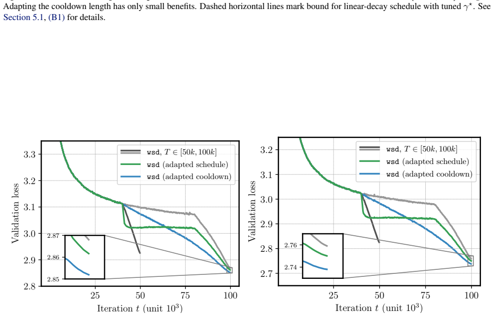
The central claim is that the last-iterate suboptimality bound for SGD on convex Lipschitz objectives, evaluated at the base learning rate that minimizes it, reproduces the empirical loss curves of cosine and wsd schedules in LLM pretraining. For wsd the paper derives a closed-form bound whose cooldown phase eliminates the logarithmic factor present for constant schedules, explaining the practical cooldown benefit. The same bound predicts that the optimal base learning rate decays like $T^{-1/2}$, that cosine's optimal rate is roughly twice wsd's, and that the ratio of optimal rates across cooldown fractions is stable across horizons; these predictions match re-analysis of real training runs and yield transfer factors such as $\gamma^\star(1)\approx e^{0.7}\gamma^\star(0.2)$ for linear cooldown. The paper also shows the drop during cooldown appears in upper bounds, worst-case lower bounds computed by semidefinite programming, and a two-dimensional non-smooth convex problem, supporting the claim that the phenomenon is not architecture-specific.
Load-bearing premise
The load-bearing premise, flagged by the paper itself in Section 6, is that the schedule-shape behavior of AdamW on non-convex transformer training is governed by a worst-case bound proven for SGD on convex Lipschitz objectives; if that transfer fails at larger scales or for AdamW-specific dynamics, the central agreement and the derived tuning rules lose their foundation.
Editorial extensions
If this is right
- If the bound is the right testbed, a fully tuned base learning rate makes linear decay the optimal schedule among the studied classes, so the optimal cooldown fraction is one.
- Continued training can be scheduled by theory: after extending a wsd run from $T_1$ to $T_2$, decreasing the schedule by a computed factor such as $\rho=0.525$ for $T_2=2T_1$ keeps the bound close to a freshly tuned linear-decay run.
- Learning-rate transfer across schedules becomes a calculable multiplier: with the optimal rate for 20% linear cooldown known, the linear-decay rate is $\gamma^\star(1)\approx e^{0.7}\gamma^\star(0.2)$, avoiding a new sweep.
- The same logic explains why cosine's cycle length of one is optimal, matching the empirical recommendation for language-model pretraining.
- The improvement from adapted continued training is worth roughly 6-8% more tokens by the paper's scaling-law estimate, corresponding to about 0.01 validation loss for the 124M and 210M models.
Reading between the lines
- Editorial inference: if the bound remains predictive beyond 210M parameters, schedule experiments could be cheaply screened against the theoretical curve before spending GPU hours, with the bound serving as a prior for candidate schedules.
- Editorial inference: the paper's analysis suggests a testable decomposition—the cooldown drop is tied to non-vanishing gradient norms; monitoring $\mathbb{E}\|g_t\|^2$ during pretraining could predict whether wsd's drop will be sharp from that curve alone.
- Editorial inference: the mirror-descent extension in the appendix hints that sign-descent-like preconditioning may admit the same last-iterate bound, which would connect the SGD-based theory to Adam's success without invoking convexity of the full network.
- Editorial inference: because the bound's schedule-shape predictions are invariant to the scale of $G$ and $D$, a direct test is to vary batch size or loss scaling and check whether the optimal rate ratios remain unchanged.
Signed reviews
Editorial analysis
A structured set of objections, weighed in public.
Referee Report
Summary. The paper studies the connection between a last-iterate suboptimality bound for non-smooth stochastic convex optimization (Defazio et al., 2023) and learning-rate schedules for large model training. It derives a bound for the wsd schedule, shows that the bound's shape over time resembles empirical validation-loss curves for cosine and wsd schedules, and uses the bound's minimizer to construct schedule-extension rules and to transfer optimal base learning-rates between schedules. The experiments include predictions for 124M and 210M Llama-type models, ImageNet ResNet50 with SGD, and OpenWebText2 language models. The paper also provides a mirror-descent extension in Appendix F and a PEP-based lower-bound analysis in Appendix B.4.
Significance. The paper offers a novel perspective on learning-rate scheduling by showing that predictions from a simple non-smooth convex bound can match empirical observations. The transfer rules and schedule-extension scheme are validated out-of-sample on real training runs, and the code is available, which is a genuine strength. However, the central link—from a worst-case SGD bound with an unmeasured gradient-norm profile to AdamW on non-convex transformers—is not fully established. Because the claimed 'surprising agreement' is the main thesis, this gap tempers the significance of the theoretical framing, even though the practical transfer rule (exp(0.7) factor) is a useful empirical contribution.
major comments (3)
- [Section 4.2, Fig. 6] The conclusion in Sections 3.1 and 4.1 that the wsd cooldown drop and the cosine/wsd comparison are reproduced by the bound relies on the assumption G_t = 1 for all t. Figure 6 shows that the sudden drop disappears when G_t is proportional to t^alpha for alpha = -0.5 or -1, and the schedule comparison changes materially. Since no gradient-norm measurements are reported for any of the LLM, ImageNet, or OpenWebText2 runs, and since AdamW is invariant to the scale of the stochastic gradient, it remains unclear whether the empirical runs satisfy the required profile. This is a load-bearing assumption for the claimed agreement, and it should be tested by measuring G_t during training or replaced by a more robust theoretical condition.
- [Section 6] The manuscript explicitly acknowledges that the theoretical results apply to SGD on convex objectives while all main experiments (Figs. 1, 10, 12 and the OpenWebText2/ImageNet replications) use AdamW or SGD on non-convex models. This gap is more than a caveat because the practical quantities used in Section 5, such as the schedule-reduction factor rho = 0.525 for T2 = 2T1 and the transfer factor exp(0.7) from Fig. 11, are derived from the convex bound. The evidence offered for transfer (the mirror-descent extension in Appendix F and references to SGD/Adam equivalence) is circumstantial. The paper should provide a direct empirical test of whether the bound's schedule-shape predictions hold for AdamW on a small transformer, or present the tuning rules as heuristics rather than theory-based rules.
- [Section 3.1, Figs. 1–3] The agreement between the theoretical bound and empirical loss curves is assessed visually, without a quantitative measure. The bound has an arbitrary vertical scale (D = G = 1) and is a worst-case upper bound rather than a model of the loss trajectory. The authors should report a quantitative summary of the match, such as the correlation between the predicted and observed curves after optimally scaling the bound, or a defined feature (e.g., the drop height) with an error bar. Without such a measure, the 'surprisingly close match' claim is difficult to evaluate and could be confounded by the many degrees of freedom in the schedules and the chosen base learning-rates.
minor comments (5)
- [Fig. 6 caption] The word 'converegnce' in the caption is a typo and should be corrected to 'convergence'.
- [Section 4.2] The phrase 'the bound of the expected gradient norms G1:T' should be 'the bound on the expected gradient norms G1:T'.
- [Theorem 3.4] The symbol '≾' is used without a definition; please specify that it denotes an asymptotic inequality as T tends to infinity.
- [Section 5.1] The statement 'we verified that changing the values of G, D, or T1 do not affect the result' is not supported by a figure or table; a one-line explanation of the multiplicative scaling would be clearer.
- [Appendix B.5] The description of the grid for base learning-rate gamma and cooldown fraction c does not mention the number of seeds or run-to-run variance, so the fitted optimum gamma*(c) in Fig. 12a has no uncertainty estimate.
Circularity Check
No significant circularity: the bound-based predictions are computed from an externally cited theorem and self-contained algebra, and the empirical comparisons use independent training data; the main limitations are assumption mismatches rather than circular reductions.
full rationale
The paper's derivation chain is not circular on the definition used in this review. Theorem 3.1 is taken from Defazio et al. (2023) and proved in Appendix E, while Corollary 3.3 and the wsd bound (Theorem 3.4/G.1) are new algebra that follows from the stated convexity and gradient-norm assumptions. The schedule-shape predictions (cosine vs. wsd curves, the approximate 2-to-1 optimal learning-rate ratio, the inverse-square-root scaling with horizon, the cooldown log-term cancellation, and the e^{0.7} transfer factor) are computed by minimizing Eq. (8) with G_t = D = 1; because these constants factor out of the minimizer for constant G_t, the predictions do not depend on fitted values. The empirical checks use loss curves from Hägele et al. (2024) and new runs on Llama-style models, ImageNet, and OpenWebText2, and none of these runs is used to set a free parameter in the bound. The clearest limitations, namely SGD theory versus AdamW practice (Section 6) and the unmeasured gradient-norm profile whose decay removes the cooldown drop (Section 4.2), are assumption mismatches rather than reductions of the prediction to its inputs. One mild methodological caveat is that the empirical transfer check in Section 5.2 estimates the optimal learning rate by fitting h_c(γ) = A_c/γ + B_cγ + C_c, whose functional form is borrowed from the bound (8); this makes the estimator share the theory's parametric shape, but the fitted coefficients A_c and B_c are free and data-determined, so the agreement is not forced by construction. Overall circularity is minimal.
Assumptions & free parameters
free parameters (3)
- Initial distance D =
1
- Gradient norm bound G =
1
- h_c coefficients (A_c, B_c, C_c) =
fitted per cooldown fraction c
assumptions (4)
- domain assumption Each loss f(.,s) is convex (A1)
- domain assumption Expected squared gradient norms are bounded by G_t^2 (A3), with G_t = G constant
- domain assumption AdamW training follows the same schedule-dependent suboptimality shape as the SGD bound
- domain assumption The convex optimization landscape is a faithful proxy for the transformer loss landscape
Cite this review
Pith. "Pith review of The Surprising Agreement Between Convex Optimization Theory and Learning-Rate Scheduling for Large Model Training." pith.science (2026). https://pith.science/paper/OUZ7MZ3Y
@misc{pith2026250118965,
  author       = {Pith},
  title        = {Pith review of: The Surprising Agreement Between Convex Optimization Theory and Learning-Rate Scheduling for Large Model Training},
  year         = {2026},
  howpublished = {\url{https://pith.science/paper/OUZ7MZ3Y}},
  note         = {Machine review of arXiv:2501.18965}
}
read the original abstract
We show that learning-rate schedules for large model training behave surprisingly similar to a performance bound from non-smooth convex optimization theory. We provide a bound for the constant schedule with linear cooldown; in particular, the practical benefit of cooldown is reflected in the bound due to the absence of logarithmic terms. Further, we show that this surprisingly close match between optimization theory and practice can be exploited for learning-rate tuning: we achieve noticeable improvements for training 124M and 210M Llama-type models by (i) extending the schedule for continued training with optimal learning-rate, and (ii) transferring the optimal learning-rate across schedules.
Figures


Figures from the paper (24 more)




Forward citations
Cited by 6 Pith papers
-
A Defense of the Quadratic Model
Local Taylor-expanded quadratic models reproduce a 150M-parameter LLM's validation loss for up to 10% of training late in the run, and LLM pretraining operates within a factor of 2 of a stochastic or deterministic edg...
-
Scaling Collapse Reveals Universal Dynamics in Compute-Optimally Trained Neural Networks
Compute-optimally trained networks of different sizes show loss curves that collapse onto one universal curve after normalization; with learning rate decay, the collapse is tighter than seed-to-seed noise, providing a...
-
AGNFormer I: Reconstruction of AGN spectra using a probabilistic transformer model
An uncertainty-aware transformer reconstructs masked AGN broad lines and spectral halves with 4-16% flux errors and beats eleven purpose-built Lyα-reconstruction algorithms on a blind benchmark.
-
WSqD: A Horizon-Free Learning Rate Schedule for Large Model Training
WSqD uses a horizon-independent shifted inverse-square-root base plus linear cooldown to get optimal last-iterate rates in convex stochastic optimization and match or beat tuned WSD on LLM pretraining with one reused ...
-
Enhancing Optimizer Stability: Momentum Adaptation of The NGN Step-size
NGN-M, a momentum variant of the NGN step-size, provably converges at O(1/sqrt(K)) under milder assumptions and shows wider step-size stability than Adam, Momo, and SGDM in vision and language tasks.
-
Why Do We Need Warm-up? A Theoretical Perspective
Under the proposed (H0,H1)-smoothness condition, gradient descent with a warm-up-style adaptive step-size provably converges faster than with any fixed step-size.
Reference graph
Works this paper leans on
-
[1]
Why you don't overfit, and don't need Bayes if you only train for one epoch
Aitchison, L. Why you don’t overfit, and don’t need Bayes if you only train for one epoch. arXiv:2411.14478, Novem- ber
-
[2]
improves over wsd, which confirms the findings of Section 5.2. For validation set metrics, we display a running average over five epoch in thick to smoothen the plot, and the original data in thin. Note that the final train loss of wsd appears slightly higher as we display the epoch-wise average of mini-batch losses; due to the steep descent of the loss a...
work page 2024
-
[7]
Loss landscape characterization of neural networks without over-parametrization
9 Learning Rate Scheduling for Large Model Training Islamov, R., Ajroldi, N., Orvieto, A., and Lucchi, A. Loss landscape characterization of neural networks without over-parametrization. arXiv:2410.12455, October
-
[12]
Rethinking conventional wisdom in machine learn- ing: From generalization to scaling
Xiao, L. Rethinking conventional wisdom in machine learn- ing: From generalization to scaling. arXiv:2409.15156, September
-
[13]
No more Adam: Learning rate scaling at initialization is all you need
Xu, M., Xiang, L., Cai, X., and Wen, H. No more Adam: Learning rate scaling at initialization is all you need. arXiv:2412.11768, December
-
[14]
Zamani, M. and Glineur, F. Exact convergence rate of the last iterate in subgradient methods. arXiv:2307.11134, July
-
[15]
• Appendix B: supplementary information on our experiments
11 Learning Rate Scheduling for Large Model Training Appendix The supplementary material is organized as follows: • Appendix A: ablation on bounds on the minimal suboptimality bounds. • Appendix B: supplementary information on our experiments. • Appendix C: additional experiments for training language and vision models • Appendix D: technical lemmas • App...
work page 2003
-
[16]
Same as Fig. 2, but with Ωt from (11) The bound on the best-so-far bound has a very different shape of the last-iterate bound. This shows that standard bounds such as in Theorem A.1 do not capture the real-world convergence observed in Hägele et al. (2024). 12 Learning Rate Scheduling for Large Model Training 10□2 10□1 Base learning-rate γ 10□1 100 Final ...
work page 2024
Show all 30 references
-
[18]
Convergence is plotted with the optimal base learning-rate γ⋆ (chosen individually for each schedule)
Comparison of various learning-rate schedules. Convergence is plotted with the optimal base learning-rate γ⋆ (chosen individually for each schedule). To the best of our knowledge, this recommendation is based mostly on empirical insights. Using the bound obtained in Theorem 3....
2022
-
[19]
Compare to Figure A1 in Hoffmann et al
Comparison of cycle lengths for the cosine schedule. Compare to Figure A1 in Hoffmann et al. (2022). B.4. Details on Lower Bound Computation We provide additional details for the simulation in Section 4.3. We compute the lower bounds with the PEPit package (Goujaud et al., 202...
2022
-
[20]
Details on Experiments in Fig
15 Learning Rate Scheduling for Large Model Training B.5. Details on Experiments in Fig. 1a and Section 5 Training details. The loss curves in Fig. 1a are an exact reproduction of the curves in (Hägele et al., 2024, Fig. 3); they are obtained from training a 210M Llama-style t...
2024
-
[23]
Dark grey marks the bound of the constant schedule
(Left) The benefit of cooldown is reflected in the absence of logarithmic terms. Dark grey marks the bound of the constant schedule. (Right) Plotting the individual terms of the bound Ωt = T1/γ + γT2 with γ = γ⋆ for the wsd schedule. The sudden drop of the bound comes from the...
-
[27]
We observe the same characteristic drop of the loss for wsd, as well as matching performance of wsd and cosine
Training three different model sizes on OpenWebText2. We observe the same characteristic drop of the loss for wsd, as well as matching performance of wsd and cosine. In each run the base learning rate of cosine is twice as large as for wsd. C.3. Computing the Bound-minimizing ...
2023
-
[28]
Optimizing the bound ΩT with respect to the schedule η1, . . . , ηT . (Left) Convergence of the value of the bound, matching the bound of a linear-decay schedule. (Right) Optimization trajectory from constant schedule (yellow) to linear-decay (purple). 21 Learning Rate Schedul...
2023
-
[29]
≤ Z t 0 1 s + 1ds ≤ tX s=1 1 s = Ht ≤ 1 + ln(t). E. Missing Proofs The following lemma will be the basic inequality for subsequently proving Theorem E.2; it is a standard result in the online learning and convex optimization literature (Zinkevich, 2003). Lemma E.1. Let 1 ≤ k ≤...
2023
-
[30]
Theorem 3.1 follows from applying Theorem E.2 with ˆηt := γηt
If one carries through this term to the end, then we obtain multiple terms in the bound that depend on ηT . Theorem 3.1 follows from applying Theorem E.2 with ˆηt := γηt. We finally prove Theorem E.2. Proof. First, apply Lemma E.1 with u → x⋆ and k → 1 to obtain TX t=1 ηtE[f (...
2003
-
[31]
From the (generalized) Cauchy-Schwarz inequality combined with Young’s inequality, we have s3 ≤ µ 2 ∥xt+1 − xt∥2 + η2 t 2µ ∥gt∥2 ∗
From (17), we have s2 = Bψ(u, xt) − Bψ(u, xt+1) − Bψ(xt+1, xt). From the (generalized) Cauchy-Schwarz inequality combined with Young’s inequality, we have s3 ≤ µ 2 ∥xt+1 − xt∥2 + η2 t 2µ ∥gt∥2 ∗. Using that −Bψ(xt+1, xt) ≤ −µ 2 ∥xt+1 − xt∥2, we obtain ηt[f (xt, st) − f (u, st)...
2023
-
[400]
For each schedule we sweep the base learning-rate γ and plot the bound Ωt for γ = γ⋆ obtained from Corollary 3.3. B.3. Cosine Cycle Length For the cosine schedule, an important hyperparameter is its cycle length, that is, the amount of training where the schedule first reaches...
2017
-
[1970]
Training trajectories, mini-batch losses and the curious role of the learning rate
Sandler, M., Zhmoginov, A., Vladymyrov, M., and Miller, N. Training trajectories, mini-batch losses and the curious role of the learning rate. arXiv:2301.02312, January
-
[1983]
Optimal linear decay learning rate schedules and further refinements
Defazio, A., Cutkosky, A., Mehta, H., and Mishchenko, K. Optimal linear decay learning rate schedules and further refinements. arXiv:2310.07831, October
-
[2003]
Chinchilla scaling: A replication attempt
Besiroglu, T., Erdil, E., Barnett, M., and You, J. Chinchilla scaling: A replication attempt. arXiv:2404.10102, April
-
[2013]
M., Cox, D
Shen, Y ., Stallone, M., Mishra, M., Zhang, G., Tan, S., Prasad, A., Soria, A. M., Cox, D. D., and Panda, R. Power scheduler: A batch size and token number agnostic learn- ing rate scheduler. arXiv:2408.13359, August
-
[2016]
We train all models with SGD with heavy-ball momentum
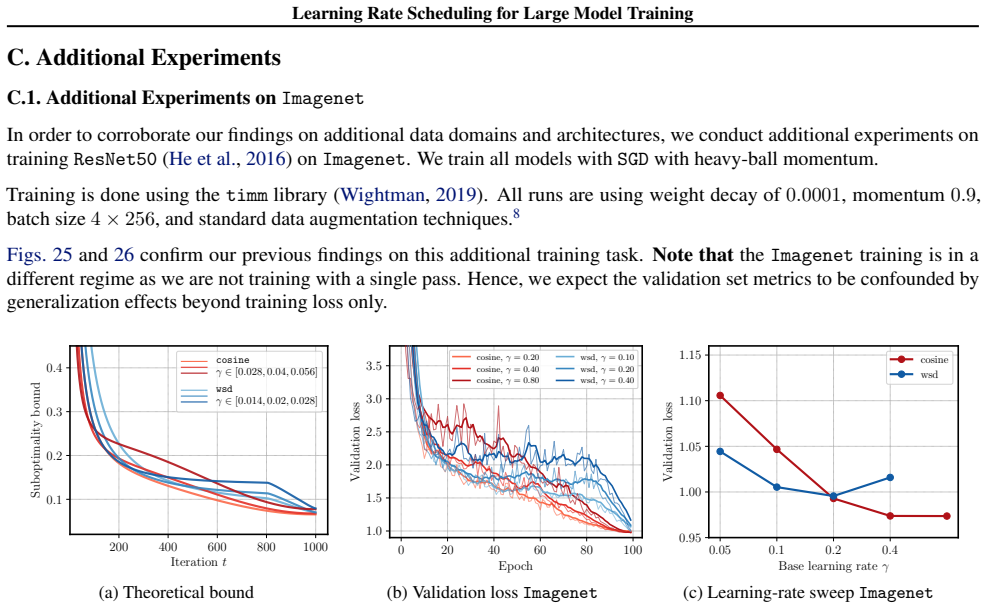
on Imagenet. We train all models with SGD with heavy-ball momentum. Training is done using the timm library (Wightman, 2019). All runs are using weight decay of 0.0001, momentum 0.9, batch size 4 × 256, and standard data augmentation techniques.8 Figs. 25 and 26 confirm our pr...
2019
-
[2018]
Deep residual learning for image recognition
He, K., Zhang, X., Ren, S., and Sun, J. Deep residual learning for image recognition. In 2016 IEEE Conference on Computer Vision and Pattern Recognition (CVPR), pp. 770–778,
2016
-
[2019]
For all further details we refer to Hägele et al
with a weight decay of 0.1. For all further details we refer to Hägele et al. (2024, App. A.1). Note that all training curves show the validation loss computed over a subset of 32 batches, while the final validation loss is computed over approx. 6 000 batches; hence, the final...
2024
-
[2020]
Rockafellar, R
[Online; accessed 08- November-2024]. Rockafellar, R. T. Convex Analysis. Princeton Mathematical Series, No
2024
-
[2021]
Brown, T., Mann, B., Ryder, N., Subbiah, M., Kaplan, J. D., Dhariwal, P., Neelakantan, A., Shyam, P., Sastry, G., Askell, A., Agarwal, S., Herbert-V oss, A., Krueger, G., Henighan, T., Child, R., Ramesh, A., Ziegler, D., Wu, J., Winter, C., Hesse, C., Chen, M., Sigler, E., Lit...
1901
-
[2022]
More concretely, assume we have trained a model of sizeN1 for D1 tokens
states that the loss L(N, D) for a model with parameters N after training for D tokens can be estimated with L(N, D) = E + A N α + B Dβ , (12) where E, A, B, α, βare usually fitted from data. More concretely, assume we have trained a model of sizeN1 for D1 tokens. To arrive at...
2024
-
[2023]
B., Hendrickx, J
Taylor, A. B., Hendrickx, J. M., and Glineur, F. Smooth strongly convex interpolation and exact worst-case per- formance of first-order methods. Mathematical Program- ming, 161(1-2):307–345, 2017a. Taylor, A. B., Hendrickx, J. M., and Glineur, F. Exact worst- case performance ...
-
[2024]
Accurate, large minibatch SGD: Training ImageNet in 1 hour
Goyal, P., Dollár, P., Girshick, R., Noordhuis, P., Wesolowski, L., Kyrola, A., Tulloch, A., Jia, Y ., and He, K. Accurate, large minibatch SGD: Training ImageNet in 1 hour. arXiv:1706.02677, June
Reviewed August 9, 2026 · model on record in the stance chip above.
Discussion (0). Continue with ORCID to comment.