REVIEW 4 major objections 5 minor 44 references
PDEfuncta: Spectrally-Aware Neural Representation for PDE Solution Modeling
T0 review · 4 major / 5 minor · reviewed 2026-08-07 · deepseek-v4-flash
Pith's one-line read A spectrally reparameterized modulation lets one shared neural network encode many high-frequency PDE solution fields and supports forward and inverse inference from the same latent codes.
desk verdict A simple and effective modulation trick for Functa-style PDE compression; the empirical claims are strong, but the spectral-bias theory is borrowed, not re-derived, and the generalization story is thin. read the letter →
The pith
A machine-rendered reading of the paper's core claim, the machinery that carries it, and where it could break.
The reading
What carries the argument
The mechanism is the layer-wise weight construction $W_k = S_k \Phi_k = (R_k + \alpha_{k,W}\cdot 1^\top)\Phi_k$, where $\Phi_k$ is a fixed Fourier basis whose rows are phase-shifted cosines at hand-picked low and high frequencies, $R_k$ is a shared base coefficient matrix across all samples, and $\alpha_{k,W}$ is the per-sample modulation produced by a small network from the latent $z$. This places each sample's weights in a predefined frequency subspace, giving better neural tangent kernel conditioning and stronger high-frequency gradients (per Theorem 1 quoted from the Fourier reparameterization literature), while keeping instance-specific adaptation cheap and letting the same $z$ drive two networks that jointly represent paired spaces.
What would settle it
Run GFM on a solution dataset whose dominant spatial frequencies fall well outside the configured $n_{\text{low}}$–$n_{\text{high}}$ band and check whether its PSNR lead over FiLM collapses; alternatively, check directly whether the Theorem 1 gradient-ratio inequality still holds when the coefficient matrix is constrained to $R + \alpha 1^\top$ rather than being free.
Extended reading notes
Core claim
The paper's central claim is that Global Fourier Modulation (GFM), the weight reparameterization $W_k = (R_k + \alpha_{k,W} 1^\top)\Phi_k$ with a fixed cosine basis $\Phi_k$, removes the spectral-bias bottleneck of modulated INRs: high-frequency modes receive stronger gradient signals than in plain or activation-space-modulated networks, so one shared backbone and a 20-dimensional latent vector can accurately encode many solution fields at once. Building on that, PDEfuncta ties two such INRs (for spaces $A$ and $U$) to the same latent vector, so a single code represents both fields and new tasks, forward or inverse, are handled by latent inference without retraining the shared weights. The paper supports this with reconstruction comparisons against Shift, Scale, and FiLM across convection, Helmholtz, Navier–Stokes, and Kuramoto–Sivashinsky data, generalization experiments on unseen convection coefficients, and operator-learning comparisons on airfoil and pipe geometry benchmarks.
Load-bearing premise
The paper's advantage rests on the fixed Fourier basis, with frequencies chosen by hand per dataset, actually covering the spectrum of every new field; the authors themselves note that performance depends on tuning the frequency ratio.
Editorial extensions
If this is right
- A single 20-dimensional latent code can compress and reconstruct multiple high-frequency PDE solution fields that Shift, Scale, and FiLM cannot represent at comparable fidelity.
- Unseen PDE coefficients become reachable by interpolating or fitting latent codes, so inference on novel parameter regimes does not require retraining the shared network.
- A shared latent vector across paired spaces yields bidirectional operators $A \to U$ and $U \to A$, so forward and inverse problems are solved by the same representation.
- The frequency-axis design gives the practitioner explicit control over the low-frequency and high-frequency mix, which can be tuned per dataset.
Reading between the lines
- The hand-picked frequencies ($n_{\text{low}}$, $n_{\text{high}}$, $n_{\text{phase}}$) are the main transfer bottleneck: if the paper's recipe is applied to datasets whose spectra are unknown, automatic frequency selection would be the natural next step.
- Because the shared basis weights and modulations are differentiable, the same latent could in principle be optimized jointly with a physics loss, turning PDEfuncta into a PINN-style solver to speed inference further; the authors do not test this.
- The claimed advantage should be read as conditional on the SIREN backbone used throughout; other activations may interact differently with the Fourier basis.
Editorial analysis
A structured set of objections, weighed in public.
Referee Report
Summary. The paper proposes Global Fourier Modulation (GFM), a modulation technique for implicit neural representations in which each layer's weight matrix is written as W_k = (R_k + alpha_{k,W} 1^T) * Phi_k, with a shared base matrix R_k, a fixed Fourier basis Phi_k, and a per-sample modulation vector alpha_k. Building on GFM, the authors introduce PDEfuncta, a Functa-style framework that encodes paired input/output solution fields with a single shared latent vector and supports bidirectional inference between the two function spaces. The empirical sections report consistent PSNR/MSE improvements over Shift, Scale, and FiLM on five PDE reconstruction benchmarks, generalization to unseen convection coefficients through latent interpolation and partial-observation fitting, and competitive or better L2 errors than several neural-operator baselines on airfoil and pipe-flow benchmarks. The theoretical discussion invokes an existing Fourier-reparameterization theorem to argue that GFM mitigates spectral bias, although the theorem is stated for a free coefficient matrix rather than GFM's constrained additive form.
Significance. If the empirical claims hold, GFM is a simple and practical modulation mechanism that improves the spectral fidelity of dataset-level INRs at modest computational overhead, and the bidirectional Functa formulation is a useful idea for compression and inverse problems in scientific machine learning. The paper's strengths include direct ablations that isolate the modulation mechanism, standard deviations reported for the main reconstruction results in Appendix F.3, clean generalization experiments on unseen PDE coefficients, and computational cost measurements in Appendix E.2. The main weaknesses are that the theoretical justification does not cover the constrained parameterization actually used, the neural-operator comparison leaves the test-time latent-inference protocol unspecified, and the paper does not report parameter-count or capacity-matched comparisons against its baselines.
major comments (4)
- [Section 3.2, Eq. (3) and Eq. (8)] The displayed dimensions in Eq. (3) are inconsistent with the rest of the paper. Section 3.1 defines Phi_k in R^{D x M}, and Section 4.1 states that the additive modulation is applied to a matrix in R^{M x D}, but Eq. (3) writes R_k in R^{d x M} and multiplies (R_k + alpha_{k,W} 1^T) in R^{d x M} by Phi_k in R^{D x M}, which is undefined unless Phi_k is transposed or the dimensions are changed. Eq. (8) repeats the same product. Since this parameterization is the paper's central mechanism, the intended dimensions must be stated unambiguously and matched to the basis construction in Appendix H, where D = (n_low + n_high) * n_phase.
- [Section 3.2, Theorem 1] The statement that GFM 'inherits the benefits of Fourier reparameterization—such as improved NTK conditioning and stronger high-frequency response (Theorem 1)' is not supported as written. Theorem 1 is an existence result for a free trainable coefficient matrix S in R^{M x D}, whereas GFM uses the constrained family S_k = R_k + alpha_{k,W} 1^T, which is a shared base matrix plus a rank-one modulation term per layer. The theorem's gradient-ratio bound does not automatically transfer to this low-dimensional affine subspace, and the paper does not re-derive it for the constrained case. The limitation is compounded by the paper's own acknowledgement in Appendix B that optimal performance depends on tuning the frequency ratio (n_low, n_high, n_phase). Please either prove an analogue of the theorem for the constrained parameterization or explicitly restate the theoretical discussion as a heuristic motivation rather than a guarantee.
- [Section 5.3.2, Table 4] The neural-operator evaluation protocol for unseen samples is not specified. A standard operator baseline such as FNO receives the input field A and predicts U in one forward pass, but PDEfuncta must obtain a latent code z for each test sample before it can decode either field. If z is found by test-time gradient fitting against the full target field U, or against A plus some other information, the comparison with one-pass neural operators is not operationally equivalent. Additionally, the text states that the authors 'evaluate both G and G† on unseen samples,' but Table 4 reports only the forward mapping G, with no numerical inverse-mapping errors. Please specify which modality is observed at test time, how z is obtained, how many inner-loop steps are used, and include the inverse-mapping results in the table.
- [Section 5.2, Table 1 and Appendix E.2] No parameter-count or capacity-matched comparison is reported against the modulation baselines. GFM's coefficient matrix S_k has D columns per layer, which can be substantially larger than the standard weight matrices used by Shift, Scale, and FiLM; for example, the Helmholtz setting uses n_low = n_high = 128 and n_phase = 32, giving D = 8192 basis vectors per layer. The gains in Table 1 could therefore partly reflect additional model capacity rather than the spectral modulation mechanism. Table 6 reports memory and time, but not parameter counts. Please report parameter counts for all modulation methods and include a capacity-matched ablation, for instance by increasing the width or depth of the baseline backbones.
minor comments (5)
- [Appendix E.1] There are several typos and grammatical issues, including 'bach size' instead of 'batch size' in Appendix E.1, 'model struggle' in Section 3.1, 'Functation space mapping' in Table 5, and 'resolution free characteristic' in the Conclusion.
- [Section 3.1, Eq. (1)] The gradient ratio in Eq. (1) is written without norms, so the expression is ambiguous; it should be stated with norms, e.g., |dL(F1)/ds_{i,m}| / |dL(F2)/ds_{i,m}|, or with a precise definition of the quotient.
- [Appendix H] Appendix H refers to 'Equation 3.1' when it means Eq. (2), and the definition T_max = 2*pi*n_low appears inconsistent with the statement in Section 3.1 that T_max is determined by the smallest frequency used; please reconcile the two descriptions.
- [Appendix J, Figure 16] The caption of Figure 16 says the results are for 'the convection equation,' but the displayed data and surrounding text concern the Helmholtz equation with coefficients (a1, a2); the caption should be corrected.
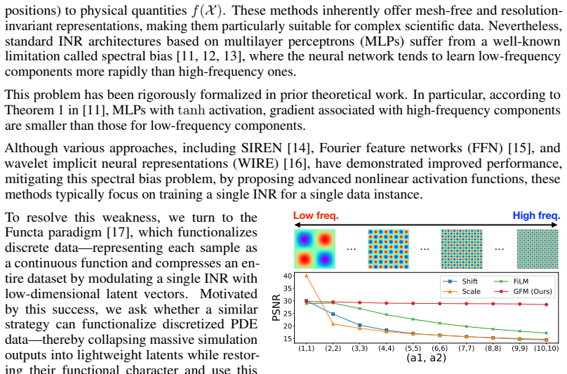
- [Figure 1] Figure 1 is referenced in the introduction but its axes and color scale are not described, and the caption does not explain how the reader should see the spectral bias from the panel; please add a clearer caption or axis labels.
Circularity Check
No circularity found: the central claims rest on genuinely out-of-sample tasks and external benchmarks; the only self-citation is a non-load-bearing data attribution, and the imported theorem is from non-author prior work.
full rationale
No significant circularity found; every load-bearing empirical claim is tested genuinely out-of-sample, and the only imported theoretical result comes from external prior work. GFM's weight construction W_k = (R_k + alpha_k,W * 1^T) * Phi_k (Eq. 3) is a constrained instance of the external Fourier reparameterization W = S * Phi from [38], so the quoted Theorem 1 (Shi, Zhou, Gu, CVPR 2024, non-author prior work) is formally applicable in shape; the paper does not re-derive the gradient bound for the additive form nor for the multi-sample meta-learning loop, which is an incompleteness of the theoretical framing, not a circular step, since the theorem's assumptions do not include the empirical results it is used to motivate. The unseen-coefficient studies (Section 5.2.1) are genuine extrapolation tests: in Setting 1 the latent for beta* is obtained by cubic interpolation of training latents with no access to the target solution, and in Setting 2 only the partial segment t in [0,0.5] is used to fit z while accuracy on the unobserved t in [0.5,1] is the reported generalization. The operator-learning results (Table 4) are evaluated against external baselines (FNO, UNet, Geo-FNO, FFNO, CORAL, MARBLE) on held-out Euler-NACA and Pipe geometries. The sole self-citation, [44] (co-author Seungjun Lee), appears only as a provenance citation for Navier-Stokes data in Appendix D.4 and is not load-bearing. The paper itself flags its own main limitation in Appendix B ('optimal performance may require careful hyperparameter tuning to select the appropriate frequency ratio'), and Appendix H confirms the frequencies are hyperparameters; this heuristic basis selection is a robustness risk for unseen spectra, but Table 1's advantage is established by direct ablation against Shift, Scale, and FiLM at matched latent dimension (20) and comparable memory, so the comparisons do not presuppose their conclusion.
Assumptions & free parameters
free parameters (4)
- Fourier basis frequency counts (n_low, n_high, n_phase) =
n_phase=32 fixed; n_high/n_low: Convection 128/32, Helmholtz 128/128, KS 64/16, NS 8/128, FWI 128/32
- Latent code dimension =
20
- Inner and outer learning rates =
eta_inner=0.01, eta_outer=0.0001
- Backbone architecture =
SIREN, 5 layers, hidden 256, modulation MLP hidden 512
assumptions (3)
- ad hoc to paper Theorem 2 of Shi et al. [38] applies to GFM's constrained coefficient matrix S = R + alpha 1^T even though it is proved for a free trainable S.
- domain assumption The fixed Fourier basis with n_low, n_high, and n_phase frequencies provides sufficient spectral coverage for every target PDE field.
- domain assumption A single 20-dimensional latent vector can jointly encode both sides of a paired function space so that bidirectional operator inference is meaningful.
Cite this review
Pith. "Pith review of PDEfuncta: Spectrally-Aware Neural Representation for PDE Solution Modeling." pith.science (2026). https://pith.science/paper/PGCCB3NG
@misc{pith2026250612790,
  author       = {Pith},
  title        = {Pith review of: PDEfuncta: Spectrally-Aware Neural Representation for PDE Solution Modeling},
  year         = {2026},
  howpublished = {\url{https://pith.science/paper/PGCCB3NG}},
  note         = {Machine review of arXiv:2506.12790}
}
read the original abstract
Scientific machine learning often involves representing complex solution fields that exhibit high-frequency features such as sharp transitions, fine-scale oscillations, and localized structures. While implicit neural representations (INRs) have shown promise for continuous function modeling, capturing such high-frequency behavior remains a challenge-especially when modeling multiple solution fields with a shared network. Prior work addressing spectral bias in INRs has primarily focused on single-instance settings, limiting scalability and generalization. In this work, we propose Global Fourier Modulation (GFM), a novel modulation technique that injects high-frequency information at each layer of the INR through Fourier-based reparameterization. This enables compact and accurate representation of multiple solution fields using low-dimensional latent vectors. Building upon GFM, we introduce PDEfuncta, a meta-learning framework designed to learn multi-modal solution fields and support generalization to new tasks. Through empirical studies on diverse scientific problems, we demonstrate that our method not only improves representational quality but also shows potential for forward and inverse inference tasks without the need for retraining.
Figures


Figures from the paper (13 more)


Reference graph
Works this paper leans on
-
[38]
Improved implicit neural representation with fourier reparameterized training
Kexuan Shi, Xingyu Zhou, and Shuhang Gu. Improved implicit neural representation with fourier reparameterized training. InProceedings of the IEEE/CVF Conference on Computer Vision and Pattern Recognition, pages 25985–25994, 2024
2024
-
[1]
SIAM, 2007
Randall J LeVeque.Finite difference methods for ordinary and partial differential equations: steady-state and time-dependent problems. SIAM, 2007
2007
-
[2]
Cambridge university press, 2002
Randall J LeVeque.Finite volume methods for hyperbolic problems, volume 31. Cambridge university press, 2002
work page 2002
-
[3]
An introduction to the finite element method.New York, 27(14), 1993
Junuthula Narasimha Reddy. An introduction to the finite element method.New York, 27(14), 1993
work page 1993
-
[4]
Workshop report on basic research needs for scientific machine learning: Core technologies for artificial intelligence
Nathan Baker, Frank Alexander, Timo Bremer, Aric Hagberg, Yannis Kevrekidis, Habib Najm, Manish Parashar, Abani Patra, James Sethian, Stefan Wild, et al. Workshop report on basic research needs for scientific machine learning: Core technologies for artificial intelligence. Technical report, USDOE Office of Science (SC), Washington, DC (United States), 2019
2019
-
[5]
Physics-informed machine learning.Nature Reviews Physics, 3(6):422–440, 2021
George Em Karniadakis, Ioannis G Kevrekidis, Lu Lu, Paris Perdikaris, Sifan Wang, and Liu Yang. Physics-informed machine learning.Nature Reviews Physics, 3(6):422–440, 2021
2021
-
[6]
Neural operators for accelerating scientific simulations and design
Kamyar Azizzadenesheli, Nikola Kovachki, Zongyi Li, Miguel Liu-Schiaffini, Jean Kossaifi, and Anima Anandkumar. Neural operators for accelerating scientific simulations and design. Nature Reviews Physics, 6(5):320–328, 2024
2024
-
[7]
Scientific machine learning through physics–informed neural networks: Where we are and what’s next.Journal of Scientific Computing, 92(3):88, 2022
Salvatore Cuomo, Vincenzo Schiano Di Cola, Fabio Giampaolo, Gianluigi Rozza, Maziar Raissi, and Francesco Piccialli. Scientific machine learning through physics–informed neural networks: Where we are and what’s next.Journal of Scientific Computing, 92(3):88, 2022
2022
Show all 44 references
-
[8]
Neural operator: Learning maps between function spaces with applications to pdes.Journal of Machine Learning Research, 24(89):1–97, 2023
Nikola Kovachki, Zongyi Li, Burigede Liu, Kamyar Azizzadenesheli, Kaushik Bhattacharya, Andrew Stuart, and Anima Anandkumar. Neural operator: Learning maps between function spaces with applications to pdes.Journal of Machine Learning Research, 24(89):1–97, 2023
2023
-
[9]
Pdebench: An extensive benchmark for scientific machine learning.Advances in Neural Information Processing Systems, 35:1596–1611, 2022
Makoto Takamoto, Timothy Praditia, Raphael Leiteritz, Daniel MacKinlay, Francesco Alesiani, Dirk Pflüger, and Mathias Niepert. Pdebench: An extensive benchmark for scientific machine learning.Advances in Neural Information Processing Systems, 35:1596–1611, 2022
2022
-
[10]
Openfwi: Large-scale multi-structural benchmark datasets for full waveform inversion.Advances in Neural Information Processing Systems, 35:6007–6020, 2022
Chengyuan Deng, Shihang Feng, Hanchen Wang, Xitong Zhang, Peng Jin, Yinan Feng, Qili Zeng, Yinpeng Chen, and Youzuo Lin. Openfwi: Large-scale multi-structural benchmark datasets for full waveform inversion.Advances in Neural Information Processing Systems, 35:6007–6020, 2022
2022
-
[11]
Understanding training and generalization in deep learning by fourier analysis
Zhiqin John Xu. Understanding training and generalization in deep learning by fourier analysis. arXiv preprint arXiv:1808.04295, 2018
2018 arXiv
-
[12]
On the spectral bias of neural networks
Nasim Rahaman, Aristide Baratin, Devansh Arpit, Felix Draxler, Min Lin, Fred Hamprecht, Yoshua Bengio, and Aaron Courville. On the spectral bias of neural networks. InInternational conference on machine learning, pages 5301–5310. PMLR, 2019
-
[13]
Overview frequency principle/spectral bias in deep learning.Communications on Applied Mathematics and Computation, pages 1–38, 2024
Zhi-Qin John Xu, Yaoyu Zhang, and Tao Luo. Overview frequency principle/spectral bias in deep learning.Communications on Applied Mathematics and Computation, pages 1–38, 2024
2024
-
[14]
Im- plicit neural representations with periodic activation functions.Advances in neural information processing systems, 33:7462–7473, 2020
Vincent Sitzmann, Julien Martel, Alexander Bergman, David Lindell, and Gordon Wetzstein. Im- plicit neural representations with periodic activation functions.Advances in neural information processing systems, 33:7462–7473, 2020
2020
-
[15]
Fourier features let networks learn high frequency functions in low dimensional domains.Advances in neural information processing systems, 33:7537–7547, 2020
Matthew Tancik, Pratul Srinivasan, Ben Mildenhall, Sara Fridovich-Keil, Nithin Raghavan, Utkarsh Singhal, Ravi Ramamoorthi, Jonathan Barron, and Ren Ng. Fourier features let networks learn high frequency functions in low dimensional domains.Advances in neural information proce...
2020
-
[16]
Wire: Wavelet implicit neural representations
Vishwanath Saragadam, Daniel LeJeune, Jasper Tan, Guha Balakrishnan, Ashok Veeraraghavan, and Richard G Baraniuk. Wire: Wavelet implicit neural representations. InProceedings of the IEEE/CVF Conference on Computer Vision and Pattern Recognition, pages 18507–18516, 2023. 10
2023
-
[17]
From data to functa: Your data point is a function and you can treat it like one.arXiv preprint arXiv:2201.12204, 2022
Emilien Dupont, Hyunjik Kim, SM Eslami, Danilo Rezende, and Dan Rosenbaum. From data to functa: Your data point is a function and you can treat it like one.arXiv preprint arXiv:2201.12204, 2022
2022 arXiv
-
[18]
Film: Visual reasoning with a general conditioning layer
Ethan Perez, Florian Strub, Harm De Vries, Vincent Dumoulin, and Aaron Courville. Film: Visual reasoning with a general conditioning layer. InProceedings of the AAAI conference on artificial intelligence, volume 32, 2018
2018
-
[19]
Deeponet: Learning nonlinear operators for identifying differential equations based on the universal approximation theorem of operators
Lu Lu, Pengzhan Jin, and George Em Karniadakis. Deeponet: Learning nonlinear operators for identifying differential equations based on the universal approximation theorem of operators. arXiv preprint arXiv:1910.03193, 2019
1910 arXiv
-
[20]
Fourier neural operator for parametric partial differen- tial equations.arXiv preprint arXiv:2010.08895, 2020
Zongyi Li, Nikola Kovachki, Kamyar Azizzadenesheli, Burigede Liu, Kaushik Bhattacharya, Andrew Stuart, and Anima Anandkumar. Fourier neural operator for parametric partial differen- tial equations.arXiv preprint arXiv:2010.08895, 2020
2010 arXiv
-
[21]
Factorized fourier neural operators
Alasdair Tran, Alexander Mathews, Lexing Xie, and Cheng Soon Ong. Factorized fourier neural operators. InThe Eleventh International Conference on Learning Representations, 2023
2023
-
[22]
Continuous pde dynamics forecasting with implicit neural representations.arXiv preprint arXiv:2209.14855, 2022
Yuan Yin, Matthieu Kirchmeyer, Jean-Yves Franceschi, Alain Rakotomamonjy, and Patrick Gallinari. Continuous pde dynamics forecasting with implicit neural representations.arXiv preprint arXiv:2209.14855, 2022
2022 arXiv
-
[23]
Gridmix: Exploring spatial modulation for neural fields in pde modeling
Honghui Wang, Shiji Song, and Gao Huang. Gridmix: Exploring spatial modulation for neural fields in pde modeling. InThe Thirteenth International Conference on Learning Representations, 2025
2025
-
[24]
Maziar Raissi, Paris Perdikaris, and George E Karniadakis. Physics-informed neural networks: A deep learning framework for solving forward and inverse problems involving nonlinear partial differential equations.Journal of Computational physics, 378:686–707, 2019
2019
-
[25]
Nerf: Representing scenes as neural radiance fields for view synthesis
Ben Mildenhall, Pratul P Srinivasan, Matthew Tancik, Jonathan T Barron, Ravi Ramamoor- thi, and Ren Ng. Nerf: Representing scenes as neural radiance fields for view synthesis. Communications of the ACM, 65(1):99–106, 2021
2021
-
[26]
Neural tangent kernel: Convergence and generalization in neural networks.Advances in neural information processing systems, 31, 2018
Arthur Jacot, Franck Gabriel, and Clément Hongler. Neural tangent kernel: Convergence and generalization in neural networks.Advances in neural information processing systems, 31, 2018
2018
-
[27]
Neural networks fail to learn periodic functions and how to fix it.Advances in Neural Information Processing Systems, 33:1583–1594, 2020
Liu Ziyin, Tilman Hartwig, and Masahito Ueda. Neural networks fail to learn periodic functions and how to fix it.Advances in Neural Information Processing Systems, 33:1583–1594, 2020
2020
-
[28]
Deepsdf: Learning continuous signed distance functions for shape representation
Jeong Joon Park, Peter Florence, Julian Straub, Richard Newcombe, and Steven Lovegrove. Deepsdf: Learning continuous signed distance functions for shape representation. InProceed- ings of the IEEE/CVF conference on computer vision and pattern recognition, pages 165–174, 2019
2019
-
[29]
Learning nonlinear operators via deeponet based on the universal approximation theorem of operators
Lu Lu, Pengzhan Jin, Guofei Pang, Zhongqiang Zhang, and George Em Karniadakis. Learning nonlinear operators via deeponet based on the universal approximation theorem of operators. Nature machine intelligence, 3(3):218–229, 2021
2021
-
[30]
Multiwavelet-based operator learning for differential equations.Advances in neural information processing systems, 34:24048–24062, 2021
Gaurav Gupta, Xiongye Xiao, and Paul Bogdan. Multiwavelet-based operator learning for differential equations.Advances in neural information processing systems, 34:24048–24062, 2021
2021
-
[31]
Wavelet neural operator: a neural operator for parametric partial differential equations.arXiv preprint arXiv:2205.02191, 2022
Tapas Tripura and Souvik Chakraborty. Wavelet neural operator: a neural operator for parametric partial differential equations.arXiv preprint arXiv:2205.02191, 2022
2022 arXiv
-
[32]
Neural operator: Graph kernel network for partial differential equations.arXiv preprint arXiv:2003.03485, 2020
Zongyi Li, Nikola Kovachki, Kamyar Azizzadenesheli, Burigede Liu, Kaushik Bhattacharya, Andrew Stuart, and Anima Anandkumar. Neural operator: Graph kernel network for partial differential equations.arXiv preprint arXiv:2003.03485, 2020
2003 arXiv
-
[33]
Learning mesh-based simulation with graph networks.arXiv preprint arXiv:2010.03409, 2020
Tobias Pfaff, Meire Fortunato, Alvaro Sanchez-Gonzalez, and Peter W Battaglia. Learning mesh-based simulation with graph networks.arXiv preprint arXiv:2010.03409, 2020. 11
2010 arXiv
-
[34]
Fourier neural operator with learned deformations for pdes on general geometries.Journal of Machine Learning Research, 24(388):1–26, 2023
Zongyi Li, Daniel Zhengyu Huang, Burigede Liu, and Anima Anandkumar. Fourier neural operator with learned deformations for pdes on general geometries.Journal of Machine Learning Research, 24(388):1–26, 2023
2023
-
[35]
Geometry-informed neural operator for large-scale 3d pdes.Advances in Neural Information Processing Systems, 36, 2024
Zongyi Li, Nikola Kovachki, Chris Choy, Boyi Li, Jean Kossaifi, Shourya Otta, Moham- mad Amin Nabian, Maximilian Stadler, Christian Hundt, Kamyar Azizzadenesheli, et al. Geometry-informed neural operator for large-scale 3d pdes.Advances in Neural Information Processing Systems...
2024
-
[36]
Operator learning with neural fields: Tackling pdes on general geometries.Advances in Neural Information Processing Systems, 36:70581–70611, 2023
Louis Serrano, Lise Le Boudec, Armand Kassaï Koupaï, Thomas X Wang, Yuan Yin, Jean-Noël Vittaut, and Patrick Gallinari. Operator learning with neural fields: Tackling pdes on general geometries.Advances in Neural Information Processing Systems, 36:70581–70611, 2023
2023
-
[37]
Spatial functa: Scaling functa to imagenet classification and generation
Matthias Bauer, Emilien Dupont, Andy Brock, Dan Rosenbaum, Jonathan Richard Schwarz, and Hyunjik Kim. Spatial functa: Scaling functa to imagenet classification and generation. arXiv preprint arXiv:2302.03130, 2023
2023 arXiv
-
[39]
An overview of full-waveform inversion in exploration geophysics.Geophysics, 74(6):WCC1–WCC26, 2009
Jean Virieux and Stéphane Operto. An overview of full-waveform inversion in exploration geophysics.Geophysics, 74(6):WCC1–WCC26, 2009
2009
-
[40]
Model-agnostic meta-learning for fast adap- tation of deep networks
Chelsea Finn, Pieter Abbeel, and Sergey Levine. Model-agnostic meta-learning for fast adap- tation of deep networks. InInternational conference on machine learning, pages 1126–1135. PMLR, 2017
2017
-
[41]
Fast context adaptation via meta-learning
Luisa M Zintgraf, Kyriacos Shiarlis, Vitaly Kurin, Katja Hofmann, and Shimon Whiteson. Fast context adaptation via meta-learning. 2019
2019
-
[42]
U-net: Convolutional networks for biomedical image segmentation
Olaf Ronneberger, Philipp Fischer, and Thomas Brox. U-net: Convolutional networks for biomedical image segmentation. InMedical image computing and computer-assisted intervention–MICCAI 2015: 18th international conference, Munich, Germany, October 5-9, 2015, proceedings, part I...
2015
-
[43]
On the benefits of memory for modeling time-dependent PDEs
Ricardo Buitrago, Tanya Marwah, Albert Gu, and Andrej Risteski. On the benefits of memory for modeling time-dependent PDEs. InThe Thirteenth International Conference on Learning Representations, 2025
2025
-
[44]
Inducing point operator transformer: A flexible and scalable architecture for solving pdes
Seungjun Lee and Taeil Oh. Inducing point operator transformer: A flexible and scalable architecture for solving pdes. InProceedings of the AAAI Conference on Artificial Intelligence, volume 38, pages 153–161, 2024. 12 A Symbol Definitions Table 5 summarizes the key symbols an...
2024
Reviewed August 7, 2026 · model on record in the stance chip above.
Discussion (0). Sign in to comment.