REVIEW 4 major objections 4 minor 26 references
Positional Encoding meets Persistent Homology on Graphs
T0 review · 4 major / 4 minor · reviewed 2026-08-07 · deepseek-v4-flash
Pith's one-line read The paper establishes that positional encodings and persistent homology are incomparable on graphs, and that its PiPE method, which feeds persistence summaries of positional encodings into message passing, is strictly more expressive than…
desk verdict The PiPE architecture is a reasonable engineering contribution, but the central proofs that it strictly beats LSPE and PH rest on false Laplacian spectra claims. read the letter →
The pith
A machine-rendered reading of the paper's core claim, the machinery that carries it, and where it could break.
The reading
What carries the argument
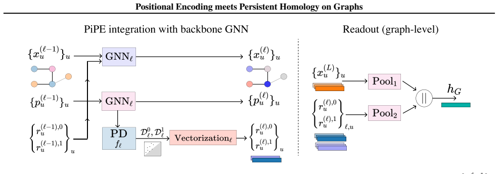
The central object is the persistence diagram of a vertex-color filtration whose colors are the current positional embeddings, computed inside the message-passing loop. At layer $\ell$, the encodings are pushed through a filtration function $f_\ell$; the 0- and 1-dimensional diagrams $D^0_\ell$ and $D^1_\ell$ are vectorized by learned maps $\Psi^0_\ell$ and $\Psi^1_\ell$ into node-level topological embeddings, which then participate in the update of the positional embeddings and of the node features (the feature vector concatenates the node, positional, and topological embeddings). The expressive-power arguments turn on two facts: the multiset of birth times in $D_0$ encodes the multiset of vertex colors, and differing numbers of connected components force different 0-dimensional diagrams. Those facts let the same machinery establish both incomparability of PE and PH and strict gains when the two are combined.
What would settle it
Compute the normalized Laplacian spectra of a 4-cycle ($\{0,1,1,2\}$) and a 6-cycle ($\{0,0.5,0.5,1.5,1.5,2\}$); the multisets differ, so the disjoint unions used in Proposition 4.1 cannot have identical $k$ smallest eigenpairs for $k \ge 2$, and checking the stated eigenpairs directly would invalidate the construction.
Extended reading notes
Core claim
On unattributed graphs, Laplacian, random-walk, and distance positional encodings are incomparable with persistent homology built from vertex-color filtrations: statement S1 gives graph pairs with the same Betti numbers but different encodings $\Phi_k$, while S2 and S3 give pairs with different $\beta_0$ or $\beta_1$ but identical encodings (Propositions 3.1 and 3.2). The paper then proves that if the positional encodings are used as the vertex colors of a filtration, the 0-dimensional persistence diagram $D_0$ preserves all the distinguishing power of the encodings (Lemma 3.3) and can separate graph pairs the encodings alone cannot (Propositions 3.4, 3.5, 3.6). PiPE operationalizes this by computing, at each message-passing layer, the 0- and 1-dimensional persistence diagrams of the current positional embeddings, vectorizing them with learned maps into topological node features, and concatenating those features into the next layer's updates. The claimed consequences are that PiPE based on Laplacian PE strictly dominates both LSPE and PH+LPE in distinguishing non-isomorphic graphs (Propositions 4.1 and 4.2), that random-walk-based PiPE still misses some 3-WL-separable pairs (Proposition 4.3), and that any k-FWL-separable pair can be separated by 0-dimensional diagrams under an explicitly constructed coloring (Proposition 4.4).
Load-bearing premise
The proof that PiPE strictly beats LSPE assumes that graph complexes built from disjoint 4-cycles and disjoint 6-cycles share the same lowest Laplacian eigenvectors; their spectra differ, so that construction needs a different witness pair or a revised argument.
Editorial extensions
If this is right
- Appending PiPE's persistence branch to Laplacian, random-walk, distance, SignNet, or SPE embeddings should strictly increase distinguishing power over the base PE alone, per Propositions 3.4, 3.5, and 4.2.
- PH methods that filter on Laplacian positional colors do not match PiPE: the cycle-versus-path construction in Proposition 4.2 gives graph pairs that PH+LPE cannot separate but a message-passing GNN can.
- Random-walk-based PiPE is not a 3-WL surrogate: the cospectral 4-regular pair of Proposition 4.3 is 2-WL-equivalent, so RW-based PiPE cannot separate it even though 3-WL can.
- Proposition 4.4 makes persistent homology a principled interface to the WL hierarchy: whenever k-FWL distinguishes two graphs, an explicit node coloring produces different 0-dimensional persistence diagrams.
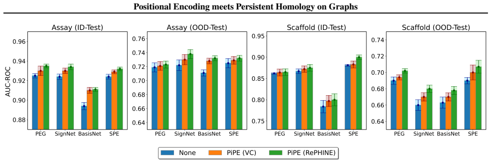
- On the reported benchmarks, adding persistent-homology vectorizations to existing positional encodings lowers test MAE on ZINC and Alchemy, raises ROC-AUC on OGBG-MOLHIV, and improves OOD-Test AUC on DrugOOD.
Reading between the lines
- The same recipe—persistence diagrams built from whatever node-level signal a model already has—could be applied to distance encodings, random feature maps, or graph-transformer attention weights, since the only requirement is a filtration over nodes.
- The empirical gains on molecular benchmarks may not rest on the strict expressivity theorems; ablating the persistence branch while keeping the extra parameters would show whether the topological summaries help as features, as regularization, or through the claimed distinguishing power.
- Since 0-dimensional diagrams already carry the component-count information behind the PE-failure examples, a natural test is whether the 1-dimensional cycle branch adds measurable value on datasets where cycles matter.
- The k-FWL result suggests a general principle: any graph invariant that yields stable colorings can be converted into a filtration that separates the same graph pairs, potentially connecting persistent homology to the full WL hierarchy.
Editorial analysis
A structured set of objections, weighed in public.
Referee Report
Summary. The manuscript proposes PiPE, a graph representation method that augments a base positional encoding (Laplacian or random-walk PE) with persistent-homology features computed from filtrations over the PE features, and integrates the result into message-passing GNNs. The theoretical portion claims (i) PE and PH are incomparable (Propositions 3.1 and 3.2); (ii) PH computed on top of PE is strictly more expressive than the base PE (Propositions 3.3–3.6); and (iii) PiPE with Laplacian PE is strictly more expressive than LSPE and than PH+LPE (Propositions 4.1 and 4.2), with additional results connecting RW-based PiPE to 3-WL (Proposition 4.3) and k-FWL to persistent-homology color-separating sets (Proposition 4.4). The empirical evaluation covers BREC expressivity, ZINC, Alchemy, OGBG-MOL*, DrugOOD, and synthetic tree tasks. The central advertised claim is that PiPE is provably more expressive than both PH and PE.
Significance. The idea of feeding PE-based persistence diagrams back into a GNN is natural, and the experimental study is substantial: the paper compares against SignNet, BasisNet, PEG, SPE, DE, and TOGL/RePHINE across several benchmarks and releases code. If the strict-expressivity theorems were correct, the paper would make a meaningful contribution to the theory of graph positional encodings. However, the definitive claims rest on proofs that contain false spectral statements (Propositions 4.1 and 4.2) and an invalid inference about k-FWL colorings (Proposition 4.4). Because the advertised contribution is precisely the provable separation, these errors are load-bearing; the empirical gains alone do not establish the paper's central claim.
major comments (4)
- [Appendix C.7, Proposition 4.1] The witness pair G=∪_{i=1}^{3n}C4 and G′=∪_{i=1}^n(C6∪C6) is claimed to satisfy Φ_k(G)=Φ_k(G′) 'having identical constant eigenvector' for all k≤12n. This is false for the normalized Laplacian Δ=I−D^{-1/2}AD^{-1/2} defined in Section 2. The multiset of eigenvalues of C4 is {0,1,1,2} and that of C6 is {0,1/2,1/2,3/2,3/2,2}. Hence G has 3n zero eigenvalues and G′ has 2n, and the first nonzero eigenvalues of the two graphs are 1 and 1/2, respectively. The k-lowest eigenpairs cannot coincide for any k>2n, and even for k≤2n the zero eigenspace dimensions differ, so no canonical choice of eigenvectors makes the encodings equal. Since this witness is the only evidence in the paper that LSPE fails on the pair, the strict-superiority conclusion of Proposition 4.1 is unsupported.
- [Appendix C.8, Proposition 4.2] For G=∪_{i=1}^n C4 and G′=∪_{i=1}^n P4, the proof asserts that 'the k smallest laplacian eigenvalues ... are all equal to 0 with the identical constant eigenvector, where k<4n'. This is false: the normalized Laplacian has exactly n zero eigenvalues (one per connected component), so for any k>n the k-lowest eigenvalues cannot all be zero, and the nonzero eigenvalues of C4 and P4 are different. The subsequent inference that PH+LPE cannot separate the pair is therefore not established. The construction may be salvageable by restricting to k≤n, but the proof as written needs to be corrected before the proposition can be accepted.
- [Appendix C.10, Proposition 4.4] The proof assumes that if k-FWL distinguishes two graphs, then there is a tuple v_w with color C∞(v_w) that does not appear in the other graph. k-FWL distinguishes graphs when the histograms of stable tuple colors differ, which can occur even when the sets of colors are identical and only the multiplicities differ. The proof also assumes 'hash functions are injective in nature', which is not guaranteed by any standard hash and is not an axiom in the paper. These two assumptions are needed to conclude that Q=∅ is a color-separating set, so the theorem is not proven.
- [Appendices C.1, C.4, C.7, C.8] Several proofs rely on the phrase 'identical constant eigenvector' for graphs with multiple connected components. For the normalized Laplacian, the zero eigenvalue has multiplicity equal to the number of connected components, and its eigenvectors are degree-normalized component indicators, not a single constant vector. The paper never specifies a canonical choice of basis for repeated eigenvalues, so equality statements of the form Φ_k(G)=Φ_k(G′) for graphs with different component counts are not well-defined. This is not a stylistic issue: the witness constructions in C.7 and C.8 choose k inside the zero eigenspace, and their validity depends on a basis convention that the paper neither states nor justifies.
minor comments (4)
- [Appendix C.1, S2/S3 and Appendix C.4] The statement that for G consisting of n/2 copies of K1∪K3 the k smallest eigenvalues are all zero for k≤n is only true for k≤n/2 when the encodings are required to come from the isolated-node components, since the triangle components contribute eigenvectors with entries 1/√3. The existence argument still works with k=n/2, but the stated range is incorrect.
- [Appendix C.5] The sentence 'have different diagrams D0(G1,Φ_k(G1), f) = D0(G2,Φ_k(G2), f)' appears to contain an equality where the intended relation is inequality, as stated in Proposition 3.6.
- [Appendix headers and Figure 1] The theorem numbering is inconsistent: Appendix C.5 is labeled 'Proof of Theorem 3.6' and C.6 is labeled 'Proof of Theorem 3.5', while the main text refers to Propositions 3.5 and 3.6; Figure 1 mixes 'Theorem' and 'Proposition' labels. Please unify the terminology.
- [Appendix C.9, Eq. (19)] The two matrices displayed for Φ_k(K) and Φ_k(K′) are not equal as arrays but are row-permutations of each other; please state explicitly that the encodings are compared as multisets of node features up to vertex relabeling.
Circularity Check
No circularity found: PiPE's derivations are self-contained special-case constructions; the flawed spectral witnesses are correctness errors, not circular reductions.
full rationale
The paper's derivation chain does not reduce to its inputs. PiPE's expressivity subsumption arguments (Proposition 4.1, Appendix C.7; Proposition 4.2, Appendix C.8) proceed by exhibiting choices of aggregation/update functions that recover LSPE or PH+LPE, which is a standard special-case argument rather than a circular definition. Strict expressivity is then attempted through witness graph pairs, relying on the elementary fact that differing numbers of connected components yield different 0-dimensional persistence diagrams; the paper cites Immonen et al. (2023) for this fact, and although that prior work shares authors (Souza, Garg), the cited theorem concerns VC filtrations and does not assume PiPE's conclusion, so it is independent support rather than a self-citation chain. Lemma 3.3 is likewise a direct corollary of prior PH theory, not a restatement of the paper's target result. No fitted parameter is relabeled as a prediction, and the empirical benchmarks are external. The most serious problems in the paper are mathematical errors, not circularity: Appendix C.7 asserts that union-of-C4 and union-of-C6 graphs have identical Laplacian PEs for k up to 12n, and Appendix C.8 makes the analogous claim for C4 versus P4, both of which are false for the normalized Laplacian because the component spectra and nullspace row norms differ. A false premise invalidates a proof without making it circular. Accordingly, the circularity score is 0.
Assumptions & free parameters
free parameters (3)
- PH embed dim =
64
- Num Filt =
8
- Hidden Filtration =
16 or 128
assumptions (4)
- standard math Persistent homology of graphs captures only 0- and 1-dimensional topological features (β0, β1) for vertex-color filtrations.
- domain assumption Message-passing GNNs with order-invariant aggregation cannot distinguish graphs with identical 1-WL colorings.
- domain assumption Theorem 1 and Lemma 5 from Immonen et al. (2023): different β0 implies different 0-dim persistence diagrams for any injective filtration; birth times encode vertex colors.
- standard math Injective hash functions exist and preserve tuple colors in Prop 4.4.
Cite this review
Pith. "Pith review of Positional Encoding meets Persistent Homology on Graphs." pith.science (2026). https://pith.science/paper/PJVVNUZX
@misc{pith2026250605814,
  author       = {Pith},
  title        = {Pith review of: Positional Encoding meets Persistent Homology on Graphs},
  year         = {2026},
  howpublished = {\url{https://pith.science/paper/PJVVNUZX}},
  note         = {Machine review of arXiv:2506.05814}
}
read the original abstract
The local inductive bias of message-passing graph neural networks (GNNs) hampers their ability to exploit key structural information (e.g., connectivity and cycles). Positional encoding (PE) and Persistent Homology (PH) have emerged as two promising approaches to mitigate this issue. PE schemes endow GNNs with location-aware features, while PH methods enhance GNNs with multiresolution topological features. However, a rigorous theoretical characterization of the relative merits and shortcomings of PE and PH has remained elusive. We bridge this gap by establishing that neither paradigm is more expressive than the other, providing novel constructions where one approach fails but the other succeeds. Our insights inform the design of a novel learnable method, PiPE (Persistence-informed Positional Encoding), which is provably more expressive than both PH and PE. PiPE demonstrates strong performance across a variety of tasks (e.g., molecule property prediction, graph classification, and out-of-distribution generalization), thereby advancing the frontiers of graph representation learning. Code is available at https://github.com/Aalto-QuML/PIPE.
Figures


Figures from the paper (5 more)




Reference graph
Works this paper leans on
-
[1]
Also, consider G′ =Q 2 ∪Q 2, with β0(G′) = 2 — consisting of two Q2 graphs, having a total of 22 + 22 nodes . Since, Q2 and Q3 are distance regular graphs (Brouwer et al., 2012), both G and G′ have the same DE-1 i.e. Φd(G) = Φd(G′) for each node in the graph with d= 1 . Therefore, distance encoding relying on shortest path distance, cannot distinguish the...
work page 2023
-
[3]
— where d denotes node degree. In both cases, the obtained diagrams for bothGandG ′ are identical, i.e., D0(G, D(G), f) = ( {(α, α),(α,∞),8×(γ, γ)}ifγ > α {8×(α, α),(γ,∞),(γ, γ)}ifγ < α (10) D0(G′, D(G′), f) = ( {(α, α),(α,∞),8×(γ, γ)}ifγ > α {8×(α, α),(γ,∞),(γ, γ)}ifγ < α (11) Thus,D 0(G, D(G), f) =D0(G′, D(G′), f)— PH relying on degree information canno...
work page 2023
-
[4]
Dwivedi, V . P. and Bresson, X. A generalization of trans- former networks to graphs.arXiv e-print:2012.09699,
arXiv 2012
-
[6]
Huang, N. T. and Villar, S. A short tutorial on the weisfeiler- lehman test and its variants. InICASSP 2021-2021 IEEE International Conference on Acoustics, Speech and Sig- nal Processing (ICASSP). IEEE,
work page 2021
-
[7]
Maskey, S., Parviz, A., Thiessen, M., Stark, H., Sadikaj, Y ., and Maron, H. Generalized laplacian positional en- coding for graph representation learning.arXiv preprint arXiv:2210.15956,
-
[8]
Nikolentzos, G., Chatzianastasis, M., and Vazirgiannis, M. What do gnns actually learn? towards understanding their representations.arXiv preprint arXiv:2304.10851,
-
[11]
12 Positional Encoding meets Persistent Homology on Graphs A. Related works Graph positional encodings.Positional encodings enhance representations in Graph Neural Networks (GNNs) (Gilmer et al., 2017; Xu et al., 2019; Velickovic et al.,
work page 2017
-
[12]
by incorporating relational information between nodes based on their positions. Several approaches have been developed to achieve this, including Laplacian-based methods that utilize the graph laplacian (Dwivedi et al., 2022; Kreuzer et al., 2021; Maskey et al., 2022; Lim et al., 2023; Wang et al., 2023; Huang et al., 2024), random walk-based techniques t...
work page 2022
Show all 26 references
-
[14]
with persistent information to obtain more powerful representations, enhancing the expressivity (Ballester & Rieck, 2024; Wang et al., 2024; Yan et al.,
2024
-
[16]
For i >0, the algorithm proceeds as, C k i+1(v) = RELABEL (C k i (v), M(v)) (6) where the multi-set M(v) ={ {C k i (ϕ1(v, w)),
two tuples v and w in V(G) k get the same color if the map vi →w i induces an isomorphism between G[v] and G[w]. For i >0, the algorithm proceeds as, C k i+1(v) = RELABEL (C k i (v), M(v)) (6) where the multi-set M(v) ={ {C k i (ϕ1(v, w)), . . . , Ck i (ϕk(v, w))|w∈V(G)} } and...
2023
-
[17]
with β0(G′) = 2, β1(G′) = 2, both having a total 10 nodes, with associated positional encodings Φk(G) and Φk(G′)based onk= 4length random walk positional encodings. The positional encodings for both the graphs are Φk(G) = 0 0.50 0 0.37 0 0.50 0 0.37 0 0.50 0 ...
2023
-
[18]
Similarly, G′ has the same eigenvalues with identical constant eigenvectors
The k smallest eigenvalues corresponding to G are all equal to 0 with the identical constant eigenvector, for k≤n . Similarly, G′ has the same eigenvalues with identical constant eigenvectors. Therefore, Laplacian PE relying on fixedksmallest eigenvalue/eigenvector pairs, cann...
2023
-
[19]
The positional encodings for both the graphs are same i.e., Φk(G) = Φ k(G′) as shown in Equation (9)
with β0(G′) = 2, β1(G′) = 2, both having a total 10 nodes, with associated positional encodings Φk(G) and Φk(G′) based on k= 4 length random walk positional encodings. The positional encodings for both the graphs are same i.e., Φk(G) = Φ k(G′) as shown in Equation (9). However...
2023
-
[22]
i.e., these two graphs cannot be separated by 2-WL but 3-WL can separate them. The positional encodings for both the graphs are Φk(K) = 0 0.25 0.62 0.14 0 0.25 0.62 0.14 0 0.25 0.62 0.14 0 0.25 0.93 0.14 0 0.25 0.93 0.14 0 0.25 0.62 0.14 0 0.25 0.62 0.14 0 0....
2023
-
[23]
To compute the Persistence Homology (PH) diagrams, we employed the learnable PH method proposed by Immonen et al
as our base model. To compute the Persistence Homology (PH) diagrams, we employed the learnable PH method proposed by Immonen et al. (2023). The PH layers operated exclusively on the position encoding features of every layer with the following specified hyperparameters in Table
2023
-
[24]
Out of distribution Prediction We adhered to the precise hyperparameters and training configuration outlined in Huang et al
Table 3: Default hyperparameters for RePHINE/VC method Hyperparameter Meaning Value PH embed dim Latent dimension of PH features 64 Num Filt Number of filtrations 8 Hiden Filtration Hidden dimension of filtration functions 16 D.2. Out of distribution Prediction We adhered to t...
2024
-
[25]
D.3. Synthetic Tree Tasks We created the synthetic tree dataset by sampling random trees of maximum depths from a discretized normal N(7,1) and followed similar training setup as described in Kogkalidis et al. (2024). We adhered to the hyper-parameters and training configurati...
2024
-
[26]
E. Tabular Results 19 Positional Encoding meets Persistent Homology on Graphs Table 4: Default hyperparameters for RePHINE/VC method Hyperparameter Meaning Value PH embed dim Latent dimension of PH features 64 Num Filt Number of filtrations 8 Hiden Filtration Hidden dimension ...
2024
-
[2017]
Persistent homol- ogy and graphs representation learning.arXiv preprint arXiv:2102.12926,
Hajij, M., Zamzmi, G., and Cai, X. Persistent homol- ogy and graphs representation learning.arXiv preprint arXiv:2102.12926,
-
[2018]
and Jena, S
Verma, Y . and Jena, S. Jet characterization in heavy ion collisions by qcd-aware graph neural networks.arXiv preprint arXiv:2103.14906,
-
[2019]
D., Xu, R., Battaglia, P., and Ho, S
Cranmer, M. D., Xu, R., Battaglia, P., and Ho, S. Learning symbolic physics with graph networks.arXiv e-print 1909.05862,
1909 arXiv
-
[2020]
and Behboodi, A
9 Positional Encoding meets Persistent Homology on Graphs Cesa, G. and Behboodi, A. Algebraic topological networks via the persistent local homology sheaf.arXiv preprint arXiv:2311.10156,
-
[2021]
from topological data analysis have made rapid strides, providing topological descriptors that augment GNNs (Cesa & Behboodi, 2023; Verma et al.,
2023
-
[2023]
Alchemy: A quantum chemistry dataset for benchmarking ai models
Chen, G., Chen, P., Hsieh, C.-Y ., Lee, C.-K., Liao, B., Liao, R., Liu, W., Qiu, J., Sun, Q., Tang, J., et al. Alchemy: A quantum chemistry dataset for benchmarking ai models. arXiv e-print :1906.09427,
1906 arXiv
-
[2024]
and Zhang, M
11 Positional Encoding meets Persistent Homology on Graphs Wang, Y . and Zhang, M. An empirical study of realized gnn expressiveness.arXiv preprint arXiv:2304.07702,
-
[2025]
and generalizability (Brilliantov et al., 2024). However, these methods have not been analyzed in regards with positional encodings in graphs, and the unification of these topological descriptors with positional encodings remains an unexplored frontier. B. WL Tests The Weisfei...
1979
Reviewed August 7, 2026 · model on record in the stance chip above.
Discussion (0). Sign in to comment.