REVIEW 3 major objections 4 minor 1 cited by
Control of neural field equations with step-function inputs
T0 review · 3 major / 4 minor · reviewed 2026-08-04 · deepseek-v4-flash
Pith's one-line read The paper derives explicit constant-in-time input formulas that steer Amari-type neural fields from any initial state to any target L^p state in a short time horizon, with endpoint error of order T^2 as T goes to zero.
desk verdict The central O(T²) error estimate is not supported: the proof misses that remainder terms scale with ||I||, and a scalar counterexample shows the endpoint error is O(T) for nonlinear f. read the letter →
The pith
A machine-rendered reading of the paper's core claim, the machinery that carries it, and where it could break.
The reading
What carries the argument
The machinery is the nonlinear flow U_t generated by the drift N(u)=−αu+μ ω*f(u) and its Fréchet derivative DU_t. The paper uses a chronological-calculus representation of the solution to write the effect of a step input as a series in the duration τ: the leading term involves the exponential of DN evaluated at the nominal trajectory endpoint, and the remainder φ_{τ,T}(I) is shown to be O(τ^3). Truncating this expansion and solving the leading-order equation yields the explicit input I_fn. The spectral condition (2.22) ensures that the operator e^{τ DN}−Id is invertible, playing the role of the non-resonance condition in finite-dimensional linear control. Lemma B.2 and Proposition B.1 supply
What would settle it
Run the synthesis in the supercritical regime (µ>µc) with a0 and a1 chosen so that 0 lies in the spectrum of DN at the required endpoint, e.g., by numerically computing the spectrum of the linearized operator for a constant state and setting µ = α/(f'(a)λ) with λ in the range of the kernel's Fourier transform; if the formula (2.27) is undefined or the endpoint error fails to scale as T^2, the claimed short-time controllability in that regime collapses. Alternatively, a direct numerical check for µ>µ1 in the 2D setting measuring the error scaling would settle whether the O(T^2) guarantee extend
Extended reading notes
Core claim
The central claim is Theorem 2.19: for p≥2, given initial state a0 and target a1, and letting U_T(a0) be the free-trajectory endpoint, if the spectrum of DN(U_T(a0)) avoids the resonance set {i 2πℓ/T}, then the explicit constant input I_fn = (e^{T DN(U_T(a0))}−Id)^{-1} DN(U_T(a0))(a1−U_T(a0)) drives the solution to a1 with endpoint error O(T^2) as T→0. Three sibling formulas—forward final-state, backward initial-state, backward nominal-state—achieve the same order. The synthesis is feedforward and reduces to the linear controllability formula when f is linear. This makes Amari-type neural fields approximately controllable between arbitrary L^p states (p≥2) in arbitrarily short time by a sing
Load-bearing premise
The explicit inputs are well-defined only when the linearized drift operator along the relevant trajectory has no eigenvalue of the form i 2πℓ/T (in particular, zero is not in its spectrum); the paper proves this automatically only in the low-coupling (subcritical) regime, not in the supercritical regime it highlights.
Editorial extensions
If this is right
- If the spectral condition holds, a single constant input computed in closed form can steer the neural field between any two L^p states (p≥2) in a time horizon T with endpoint error O(T^2).
- The four explicit formulas (2.27), (3.2), (3.4), (3.6) are generically distinct but share the same accuracy order, giving practitioners a choice of which trajectory to linearize around.
- In the subcritical coupling regime μ<μ0 (μ<μ1 when p=2), the spectral conditions are automatically satisfied, so the syntheses are unconditionally valid.
- When the transfer function is linear, the construction reduces to the standard constant-input controllability formula for the linearized equation.
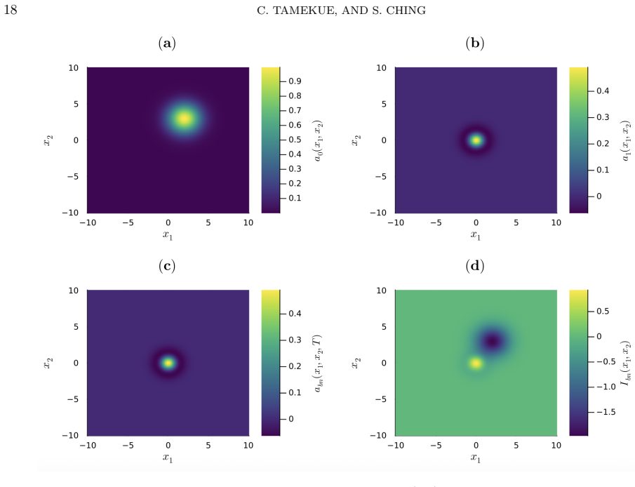
- Numerical experiments in one and two dimensions confirm the predicted O(T^2) scaling and show the explicit inputs outperform inputs obtained by linearizing at the initial or target state when those states are not equilibria.
Reading between the lines
- The O(T^2) accuracy comes with an input magnitude that grows like 1/T (since (e^{T DN}−Id)^{-1} ≈ O(1/T)); a testable quantitative tradeoff between speed, accuracy, and stimulus amplitude is implicit in the formulas and could be made explicit.
- The framework's dependence on the flow representation suggests a natural extension to bounded domains or inhomogeneous kernels without changing the synthesis structure; a numerical verification of the error rate in those settings would be a cheap next step.
- The paper motivates the supercritical regime µ>µc as a target application (spontaneous pattern formation), but its automatic invertibility guarantees stop at subcritical µ; the most valuable follow-up would be to establish or test the spectral conditions in the pattern-forming regime.
- For the visual-illusion application, the same formulas give an explicit route to synthesize a stimulus that produces a desired percept in a specified time; comparing such a synthesized input to the known inducing stimulus in the Billock–Tsou experiment would be a direct experimental falsifier.
Editorial analysis
A structured set of objections, weighed in public.
Referee Report
Summary. The paper studies approximate steering of Amari-type neural field equations (NF) by constant or step-function inputs. It proposes two lines of synthesis: a Banach fixed-point iteration (Theorem 2.4) and, as its main contribution, four explicit 'generic' input formulas — forward nominal (2.27), forward final-state (3.2), backward initial-state (3.4), and backward nominal (3.6) — claimed to drive the state to a prescribed target with endpoint error O(T^2) as the time horizon T→0, under spectral non-resonance conditions. The derivation is based on chronological-calculus representations of the flow (Theorems 2.9–2.10), an expansion (F1) of the solution for a step input, and a leading-order expansion of a remainder operator φ (Proposition 2.18). Numerical experiments in one and two dimensions are reported for subcritical parameter values. The paper also discusses applications to visual illusion prediction and tDCS.
Significance. If the O(T^2) endpoint estimate were correct, the paper would give a practically useful, explicit feedforward synthesis for controlling nonlinear neural fields in short time, with a clear comparison against linearized inputs. The use of dual flow representations, the explicit formulas (2.27), (3.2), (3.4), (3.6), and the reproducible Julia experiments are definite strengths. However, the central technical claim — that the remainder in Proposition 2.18 is O(τ^3) uniformly enough to yield O(τ^2) endpoint error with the synthesized input — is false. A one-dimensional scalar counterexample satisfying all assumptions produces an O(T) endpoint error, so the main theorems do not hold as stated. The advertised supercritical regime is also not covered by the proven spectral conditions, and the numerical tests all remain subcritical.
major comments (3)
- [§2.2.3, Theorem 2.19 and Proposition 2.18] The O(τ^3) remainder in (2.25) is not uniform in the input I. Lemma A.1 bounds φ_{τ,T}(I) by C τ^3 with C depending on ∥I∥_p (see (A.15)–(A.20)). The synthesized input I_fn in (2.27) has norm O(τ^{-1}), since (e^{τΦ}−Id)^{-1}Φ = τ^{-1}Id + O(1). Hence the discarded remainder, after substitution into (2.30), contributes O(τ), not O(τ^2), to the endpoint mismatch. This is not a technical gap but a genuine nonlinear effect: only DN appears in the input formula, so the second-order term of N cannot be cancelled. Concretely, take the scalar dynamics ẋ=N(x)+I with N(x)=−αx+μΩf(x), a0=0, a1=1, f''(0)≠0, N'(0)≠0; all Assumptions 1.2 and the spectral condition (2.22) hold. Direct Taylor expansion gives x(T)=1+(N''(0)/6)T+O(T^2), contradicting (2.29).
- [§3.1, Proposition 3.1] The same non-uniform-remainder issue invalidates the O(T^2) claims for the forward final-state input I_f, backward initial-state input I_b, and backward nominal-state input I_bn. Each of the formulas (3.2), (3.4), (3.6) contains a factor (e^{TDN}−Id)^{-1}DN = O(T^{-1}), so the second-order Taylor remainder of the nonlinear drift produces an O(T) endpoint error, not O(T^2). The proof is omitted ('omitted for brevity'), but the scalar counterexample from Theorem 2.19 applies verbatim to these formulas in the case of constant states. The proposition therefore does not provide the claimed accuracy.
- [§2.2.3, §3.2, and §6] The spectral conditions (2.22), (3.1), (3.3), (3.5) are verified only in the subcritical regime: μ<μ0 (μ<μ1 when p=2), as stated in Lemma 2.8 and Remark 2.17. The introduction and Section 5 motivate the synthesis for critical/supercritical regimes (μ≈μc or μ>μc), where patterns would not arise spontaneously. No theorem establishes invertibility in that regime, and all numerical experiments use μ<μc (e.g., μ=0.5, μ=0.624, μ=0.6). Thus the advertised application to supercritical pattern generation is not supported by the analysis.
minor comments (4)
- [Figure 3 caption] The caption mentions 'I_a0 and I_a0'; the second should be 'I_a1'.
- [§2.2.2, Remark 2.15] The operators β_{τ,T}(I), η_{τ,T}(I), ζ_{τ,T}(I) are introduced in (F2), (B1), (B2) without definition or convergence statement. If they are merely placeholders, this should be stated explicitly.
- [Definition 2.2 vs. main results] Definition 2.2 defines exact step controllability, but Theorems 2.19 and Proposition 3.1 only establish approximate steering with an error bound. The terminology should distinguish exact and approximate controllability to avoid overstatement.
- [§3.1] Proposition 3.1 is a main result but its proof is omitted entirely. Even apart from the technical error above, the omitted proof makes the claimed O(T^2) bounds unverifiable; at minimum the proof should be included or a detailed reference provided.
Circularity Check
No circularity: the control syntheses are derived in-paper from flow expansions and remainder estimates; self-citations supply standard prior facts rather than defining the target result.
full rationale
No circular step is present. The main synthesis formulas (2.27), (3.2), (3.4), and (3.6) are derived in this paper from the solution expansions (F1), (F2), (B1), and (B2), with the remainder estimates in Proposition 2.18 and Appendix A, and the operator estimates in Appendix B. No quantity is fitted to data, and no 'prediction' reduces to an assumed value of the same quantity. The O(T^2) endpoint error claim is a quantitative theorem whose proof can be inspected from equations (2.25)-(2.30); even if the skeptic's objection about non-uniform remainder constants were valid, that would be a correctness/rigor concern, not circularity, because the input is not defined in terms of the endpoint error. Citations to [50] and [47] are used for standard flow/differentiability facts and for the finite-dimensional precedent; these are prior published mathematical results, not assumptions of the conclusion, and the paper re-proves several critical lemmas in Appendices A-B. Thus the derivation chain does not collapse into its own inputs.
Assumptions & free parameters
free parameters (2)
- µ (numerical coupling strength) =
0.5 (1D ex.1), 0.624 (1D ex.2), 0.6 (2D)
- c1_1 λ and c0_3 (bump approximation coefficients) =
0.0625 and −2
assumptions (5)
- domain assumption Assumptions 1.2: f∈C^2 with f′,f′′ bounded, f(0)=0, ∥f′∥∞=1; kernel ω∈S(R^d); µ bounded by spectral stability thresholds.
- standard math Global well-posedness and invertible flow of (NF) (Prop 2.3, [54], [50, Lemma B.10]).
- domain assumption Spectral non-resonance conditions (2.22), (3.1), (3.3), (3.5): 0 not in the spectrum of the relevant DN at the relevant flow point, so (e^{T DN}−Id) and (Id−e^{−T DN}) are invertible.
- standard math The remainder operator φ_{τ,T}(I) obeys the O(τ^3) bound (A.15) with constants depending on a0, I, and the trajectory a_τ(T−t).
- domain assumption Numerical domain truncation: simulations on Ω=[−L,L] (or square) with uniform grids approximate the R^d problem without boundary-condition discussion.
Cite this review
Pith. "Pith review of Control of neural field equations with step-function inputs." pith.science (2026). https://pith.science/paper/PUEEHNJU
@misc{pith2026251022022,
  author       = {Pith},
  title        = {Pith review of: Control of neural field equations with step-function inputs},
  year         = {2026},
  howpublished = {\url{https://pith.science/paper/PUEEHNJU}},
  note         = {Machine review of arXiv:2510.22022}
}
read the original abstract
Wilson-Cowan and Amari-type models capture nonlinear neural population dynamics, providing a fundamental framework for modeling how sensory and other exogenous inputs shape activity in neural tissue. We study the controllability properties of Amari-type neural fields subject to piecewise/constant-in-time inputs. The model describes the time evolution of the polarization of neural tissue within a spatial continuum, with synaptic interactions represented by a convolution kernel. We study the synthesis of piecewise/constant-in-time inputs to achieve two-point boundary-type control objectives, namely, steering neural activity from an initial state to a prescribed target state. This approach is particularly relevant for predicting the emergence of paradoxical neural representations, such as discordant visual illusions that occur in response to overt sensory stimuli. We first present a control synthesis based on the Banach fixed-point theorem, which yields an iterative construction of a constant-in-time input under minimal regularity assumptions on the kernel and transfer function; however, it exhibits practical limitations, even in the linear case. To overcome these challenges, we then develop a generic synthesis framework based on the flow of neural dynamics drift, enabling explicit piecewise constant and constant-in-time inputs. Extensive numerical results in one and two spatial dimensions confirm the effectiveness of the proposed syntheses and demonstrate their superior performance compared to inputs derived from naive linearization at the initial or target states when these states are not equilibria of the drift dynamics. By providing a mathematically rigorous framework for controlling Amari-type neural fields, this work advances our understanding of nonlinear neural population control with potential applications in computational neuroscience, psychophysics, and neurostimulation.
Figures


Forward citations
Cited by 1 Pith paper
-
Stabilizability of neural fields from thick subsets
Linearized Amari neural fields are open-loop stabilizable from thick control sets when interaction strength is not too large relative to decay, yielding closed-loop feedback stabilizability in L2.
Reference graph
Works this paper leans on
-
[1]
Agrachev and R
[1]A. Agrachev and R. V. Gamkrelidze,The exponential representation of flows and the chronological calculus, Mathematics of the USSR-Sbornik, 35 (1979), p
1979
-
[6]
Coombes and C
[21]S. Coombes and C. Laing,Delays in activity-based neural networks, Philosophical Transactions of the Royal Society A: Mathematical, Physical and Engineering Sciences, 367 (2009), pp. 1117–1129. [22]R. Curtu and B. Ermentrout,Pattern formation in a network of excitatory and inhibitory cells with adaptation, SIAM Journal on Applied Dynamical Systems, 3 (...
2009
-
[67]
MacKay,Visual effects of non-redundant stimulation, Nature, 192 (1961), pp
[36]D. MacKay,Visual effects of non-redundant stimulation, Nature, 192 (1961), pp. 739–740. [37]D. M. MacKay,Moving visual images produced by regular stationary patterns, Nature, 180 (1957), pp. 849–850. [38]M. Nashed and L. B. Rall,Nonlinear functional analysis and applications, Differentiability and Related Properties of Nonlinear Operators: Some Aspect...
1961
-
[87]
[3]A. M. Annabi, J.-B. Pomet, D. Prandi, and L. Sacchelli,Activity estimation via distributed measurements in an orien- tation sensitive neural fields model of the visual cortex, Mathematics of Control, Signals, and Systems, (2025), pp. 1–31. [4]A. Asadi, M. Madadi Asl, A. V alizadeh, and M. Perc,Dynamics of parkinsonian oscillations mediated by transmiss...
2025
-
[307]
Grossberg, E
[29]S. Grossberg, E. Mingolla, and W. D. Ross,Visual brain and visual perception: how does the cortex do perceptual grouping?, Trends in neurosciences, 20 (1997), pp. 106–111. [30]S. Grover, W. Wen, V. Viswanathan, C. T. Gill, and R. M. Reinhart,Long-lasting, dissociable improvements in working memory and long-term memory in older adults with repetitive n...
1997
-
[353]
[24]G. B. Ermentrout and J. D. Cowan,A mathematical theory of visual hallucination patterns, Biological cybernetics, 34 (1979), pp. 137–150. 28C. TAMEKUE, AND S. CHING [25]O. F augeras, F. Grimbert, and J.-J. Slotine,Absolute stability and complete synchronization in a class of neural fields models, SIAM Journal on applied mathematics, 69 (2008), pp. 205–...
1979
-
[727]
Amari,Dynamics of pattern formation in lateral-inhibition type neural fields, Biological cybernetics, 27 (1977), pp
[2]S.-i. Amari,Dynamics of pattern formation in lateral-inhibition type neural fields, Biological cybernetics, 27 (1977), pp. 77–
1977
-
[744]
[10]M. Bolelli and D. Prandi,Neural field equations with time-periodic external inputs and some applications to visual pro- cessing, J Math Imaging Vis, 67 (2025), p. 47, https://doi.org/10.1007/s10851-025-01257-7. [11]P. C. Bressloff,Spatiotemporal dynamics of continuum neural fields, Journal of Physics A: Mathematical and Theoretical, 45 (2011), p. 0330...
Show all 15 references
-
[2004]
Tamekue, R
[47]C. Tamekue, R. Chen, and S. Ching,On the control of recurrent neural networks using constant inputs, IEEE Transactions on Automatic Control, (2025), pp. 1–16, https://doi.org/10.1109/TAC.2025.3615934. [48]C. Tamekue, D. Prandi, and Y. Chitour,Reproducing sensory induced ha...
2025
-
[2009]
Veltz,Interplay between synaptic delays and propagation delays in neural field equations, SIAM Journal on Applied Dynamical Systems, 12 (2013), pp
[53]R. Veltz,Interplay between synaptic delays and propagation delays in neural field equations, SIAM Journal on Applied Dynamical Systems, 12 (2013), pp. 1566–1612. [54]R. Veltz and O. F augeras,Local/global analysis of the stationary solutions of some neural field equations,...
2013
-
[2010]
F aye, J
[27]G. F aye, J. Rankin, and P. Chossat,Localized states in an unbounded neural field equation with smooth firing rate function: a multi-parameter analysis, Journal of mathematical biology, 66 (2013), pp. 1303–1338. [28]J. Fraser,A new visual illusion of direction, British Jou...
2013
-
[2011]
[44]E. L. Schwartz,Spatial mapping in the primate sensory projection: analytic structure and relevance to perception, Biological cybernetics, 25 (1977), pp. 181–194. [45]T. F. Sequeira and P. M. Lima,Numerical simulations of one-and two-dimensional stochastic neural field equa...
1977
-
[2012]
[42]M. Rule, M. Stoffregen, and B. Ermentrout,A model for the origin and properties of flicker-induced geometric phosphenes, PLoS computational biology, 7 (2011), p. e1002158. [43]S. J. Schiff,Neural control engineering: the emerging intersection between control theory and neu...
2011
-
[2013]
[17]B. J. Cook, A. D. Peterson, W. Woldman, and J. R. Terry,Neural field models: A mathematical overview and unifying framework, Mathematical Neuroscience and Applications, 2 (2022). [18]S. Coombes,Waves, bumps, and patterns in neural field theories, Biological cybernetics, 93...
2022
-
[2022]
Kitaoka, B
[33]A. Kitaoka, B. Pinna, and G. Brelstaff,Contrast polarities determine the direction of caf´ e wall tilts, Perception, 33 (2004), pp. 11–20. [34]C. R. Laing, W. C. Troy, B. Gutkin, and G. B. Ermentrout,Multiple bumps in a neuronal model of working memory, SIAM Journal on App...
2004
Reviewed August 4, 2026 · model on record in the stance chip above.
Discussion (0). Sign in to comment.