REVIEW 1 major objections 4 minor 1 cited by
Dynamical systems approach and cosmological attractors in newer general relativity
T0 review · 1 major / 4 minor · reviewed 2026-08-07 · deepseek-v4-flash
Pith's one-line read For one teleparallel gravity family, vacuum cosmology never accelerates
desk verdict Solid vacuum phase-space analysis with a real overstatement: the type 1 'no acceleration' claim fails at epsilon = -1, where the paper's own undetermined-H branches admit de Sitter solutions. read the letter →
The pith
A machine-rendered reading of the paper's core claim, the machinery that carries it, and where it could break.
The reading
What carries the argument
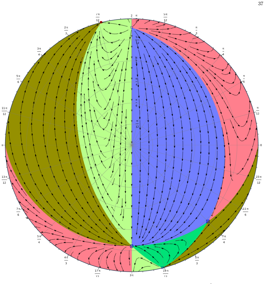
The central object is the projective decomposition of the homogeneous quadratic system dot(z) = f(z, z): writing z = Z n separates the angular dynamics of the direction n from the radial dynamics of the magnitude Z. Projective fixed points, directions n with dot(n) = 0, satisfy dot(Z) = N* $Z^{2}$, whose explicit solution Z(t) = 1 / [N*(t0 - t)] turns a positive radial rate N* into a future finite-time singularity and a negative one into a past finite-time singularity, while N* = 0 gives eternal expansion or contraction. Antipodal projective fixed points have opposite stability and opposite radial sign, and this pairing determines which directions act as attractors or repellers in expanding versus contracting universes.
What would settle it
Include a dust or radiation fluid and re-derive the type-2 phase space; if the condition w_lambda <= -1 or the big-rip attractor disappears, the paper's vacuum scenarios would not describe a matter-dominated universe. Alternatively, evolve linear perturbations about a type-2 expanding background and look for ghost or strong-coupling instabilities.
Extended reading notes
Core claim
The paper establishes that, in the vacuum, spatially flat FLRW sector, the cosmological dynamics of newer general relativity is a homogeneous quadratic dynamical system. This structure lets the authors split every solution into radial and angular parts and classify all asymptotic behaviors by projective fixed points. For type 1 theories they obtain the complete set of vacuum cosmological solutions and show that none accelerates. For type 2 theories the sign of the single parameter epsilon fixes the effective dark energy barotropic index: epsilon > 0 gives w_lambda <= -1 everywhere (phantom, no turnaround, inevitable future big rip), while epsilon < 0 gives w_lambda >= -1 (non-phantom; expanding solutions either approach H -> 0 forever or turn around to a big crunch). The barotropic index never crosses the phantom divide dynamically.
Load-bearing premise
The physical conclusions assume that vacuum, spatially flat, three-branch solutions capture the late-time dynamics of the real universe; if matter coupling or perturbations change the attractor structure, the predicted fates would not apply.
Editorial extensions
If this is right
- Type 1 theories have no accelerated vacuum solution, so by themselves they cannot explain the observed late-time acceleration; some additional dark-energy sector would be needed.
- For type 2 with epsilon > 0 the universe can only bounce and then hit a big rip; a turnaround is impossible.
- For type 2 with epsilon < 0 every expanding solution either expands forever with the Hubble parameter approaching zero or turns around and ends in a big crunch.
- The sign of epsilon fixes whether the effective dark energy is phantom or non-phantom; the barotropic index cannot dynamically cross w = -1.
- The existence of a non-hyperbolic saddle at H = 0 and antipodal attractor-repeller pairs means the qualitative fate is decided by the sign of the Hubble parameter and the theory parameter.
Reading between the lines
- If dust or radiation is added, the attractor structure could shift, since the vacuum analysis relies on matter being negligible at late times; redoing the phase space with a barotropic fluid would test whether these fates survive.
- The paper's own references flag ghost and strong-coupling pathologies in symmetric teleparallel perturbations; if those apply to the type-2 backgrounds, the vacuum attractors may be unstable even though the background derivation is consistent.
- The homogeneous quadratic projective method is not tied to newer general relativity; the same attractor classification could be applied to other teleparallel or modified-gravity cosmologies whose field equations have the same algebraic form.
- One could compare the epsilon < 0 expanding branches with observations: those are the only type-2 scenarios that allow eternal expansion with decaying Hubble parameter, so they are the natural candidates for a viable cosmology.
Editorial analysis
A structured set of objections, weighed in public.
Referee Report
Summary. The manuscript develops a dynamical-systems treatment of vacuum, spatially flat Friedmann-Lemaître-Robertson-Walker cosmology in newer general relativity, using the three spatially flat branches of homogeneous and isotropic symmetric teleparallel connections. It derives generic first-order dynamical systems, identifies degenerate parameter regions, and introduces a radial/angular decomposition that reduces the asymptotic analysis to projective fixed points, their stabilities, and the sign of the radial growth rate. The formalism is then applied to two one-parameter families selected by post-Newtonian and ghost constraints. For type 1 theories the authors claim to have found the complete set of vacuum cosmological solutions and that none of them exhibits accelerated expansion. For type 2 theories they claim that the sign of epsilon decides between phantom behavior (epsilon > 0, with any expanding solution ending in a future finite-time singularity) and non-phantom behavior (epsilon < 0, with eternal decelerated expansion or a turnaround to a big crunch). The effective dark-energy barotropic index is computed for each branch. The paper explicitly defers matter coupling and cosmological perturbations to future work.
Significance. If the analysis is correct, the paper provides a rare complete classification of vacuum cosmological attractors for a modified-gravity family with viable post-Newtonian and ghost properties, and the epsilon-sign dichotomy in type 2 theories is a sharp, falsifiable statement. Strengths of the manuscript are its explicit derivations from the field equations, the parameter-free classification in terms of the single parameter epsilon, and the self-contained formulation of the projective decomposition and radial dynamics. The type-1 no-acceleration claim, however, is contradicted by the exceptional epsilon = -1 branches identified in the same analysis, so the 'complete solution set' statement is not correct as it stands and requires qualification before the paper can be accepted.
major comments (1)
- [Section IVA, Eqs. (78)-(84); Section IVB, Eqs. (85)-(91); Section VI] The Section VI conclusion that type 1 theories contain no accelerated vacuum solutions is internally inconsistent with the epsilon = -1 exceptional branches found in Section IV. For epsilon = -1, branch 2 admits K = -2H (Eq. (82)) and branch 3 admits K = 2H (Eq. (89)), and in both cases the remaining field equation is satisfied identically once L is eliminated through \dot H = H L. Taking H(t) = H0 > 0 constant and L = 0 gives K = -2H0 for branch 2 and K = 2H0 for branch 3; the scale factor is a(t) = e^{H0 t}, with \ddot a/a = H0^2 > 0, so these are accelerated vacuum solutions. The manuscript excludes only epsilon = 0 in Section IV, not epsilon = -1, so these solutions lie inside the stated scope. The claim 'we have found the complete set of vacuum cosmological solutions, and shown that none of them exhibits any accelerated expansion' is therefore false unless epsilon = -1 is explicitly excluded or the undetermined-H branches are shown to be unphysical or otherwise discarded.
minor comments (4)
- [Eq. (88)] The printed equation (88) appears to have a sign/typesetting error: substituting a1 = 1, a2 = 0, a3 = 0, a4 = epsilon into Eq. (25b) gives -2 \dot H - 3H^2 - epsilon K(3K/4 + L) = 0, not the expression with '-3H^2 epsilon K(...)' as printed. This should be corrected for consistency with the subsequent identity for epsilon = -1, K = 2H.
- [Abstract and Section VI] The abstract contains the grammatical error 'It turns that' and should read 'It turns out'; Section VI similarly contains 'a number of phase diagram' and should read 'a number of phase diagrams'.
- [Section IVB, text before Eq. (88)] The phrase 'which in this case reads' is used twice in consecutive sentences; the second occurrence should be reworded to avoid repetition.
- [Section VI] The conclusion should explicitly state that the type-1 no-acceleration result excludes the epsilon = -1 exceptional branches, or should present an argument for why those branches are not considered physical solutions, rather than leaving this qualification implicit.
Circularity Check
No circularity: the cosmological results are derived from the field equations; self-citations are non-load-bearing classification and viability inputs.
full rationale
The derivation chain is self-contained. The paper starts from the quadratic nonmetricity action (4), derives the cosmological field equations (17)-(20), and reduces them by direct algebra to the first-order dynamical systems (27)-(29) and to the degenerate constraints of Sec. IIIB. No parameter is fitted to the target statements, and the target results are not inserted as inputs. For type 2, the effective barotropic index (97)-(99) is obtained by substituting the derived expressions for the time derivative of H into the definition (76); the sign statements w_lambda <= -1 and w_lambda >= -1, and the associated big-rip, big-crunch, and eternal-expansion scenarios, follow from the resulting equations rather than from an ansatz. The citations that carry the classification of the theory families (post-Newtonian limit [27], ghost freedom [36], branch structure [32]) are parameter-free prior derivations with no overlap of target content, so they do not import the cosmological conclusions. A correctness caveat, not a circularity, is that Section VI's claim that no type-1 solution accelerates is not entailed by the preceding derivation: for epsilon = -1, Eqs. (82) and (89) make the final equation an identity and leave H undetermined, so constant H > 0 gives an accelerated vacuum solution within the paper's own spatially flat three-branch setting. This affects the validity of the conclusion but is not a reduction of the derivation to its inputs.
Assumptions & free parameters
free parameters (1)
- epsilon (epsilon) in type 1 and type 2 theories
assumptions (4)
- domain assumption The homogeneous and isotropic symmetric teleparallel connection is fully described by branches (12)-(14) with a single function K(t) for spatially flat cosmologies.
- domain assumption Vacuum approximation: matter density and pressure are set to zero, motivated by late-time dark energy dominance.
- standard math Standard existence and stability theory for autonomous ODE systems, including linearization at fixed points and the radial/angular decomposition for homogeneous quadratic vector fields.
- domain assumption The type 1 and type 2 subclasses defined by (5) and (6) are the phenomenologically viable ones, based on prior post-Newtonian and ghost analyses.
Cite this review
Pith. "Pith review of Dynamical systems approach and cosmological attractors in newer general relativity." pith.science (2026). https://pith.science/paper/PWVXJMRD
@misc{pith2026250516917,
  author       = {Pith},
  title        = {Pith review of: Dynamical systems approach and cosmological attractors in newer general relativity},
  year         = {2026},
  howpublished = {\url{https://pith.science/paper/PWVXJMRD}},
  note         = {Machine review of arXiv:2505.16917}
}
read the original abstract
We study the cosmological dynamics of a class of symmetric teleparallel gravity theories known as ``newer general relativity'' using the methods of dynamical systems, restricted to the case of vacuum solutions with a spatially flat Friedmann-Lema\^itre-Robertson-Walker metric. For the most general class of theories, we study generic properties of the solutions, in particular their fixed points, asymptotic behavior and effective dark energy. We then apply this approach to two phenomenologically motivated subclasses of theories, which we study in full detail. For these theories, we derive the complete space of solutions and cosmological attractors, which we display in a number of phase diagram. Depending on the particular theory at hand, we find different possible scenarios, including a turnaround followed by a big crunch, a big rip and an eternally expanding universe whose Hubble parameter asymptotically approaches zero. It turns that this different behavior can be explained by the effective dark energy barotropic index, which shows either phantom or non-phantom behavior, depending on the theory, but does not change dynamically between these two possibilities.
Figures


Figures from the paper (13 more)



Forward citations
Cited by 1 Pith paper
-
Degrees of freedom of a quadratic scalar-nonmetricity theory
In quadratic scalar-nonmetricity gravity, Hamiltonian analysis shows 10, 8, and 8 degrees of freedom for cases II, V, and VI, while linear cosmological perturbation theory sees only 10, 6, and 5, indicating hidden str...
Reference graph
Works this paper leans on
-
[1]
Branch 1 We start with the first branch, where we will assumeC̸= 0, since otherwise the dynamical equations will trivially vanish. Inserting the parametrization (31) and dividing byC, the dynamical equations (21) become 3H 2 cos2 α+ 2 ˙Ksin 2 α+K(6H+K) sin 2 α+ √ 3 ˙Hsin 2α+ √ 3H(3H+K) sin 2α= 0,(32a) −2 ˙Hcos 2 α−3H 2 cos2 α+K 2 sin2 α− ˙Ksin 2α√ 3 = 0.(...
-
[2]
In this case we find the constraint √ 3Hcosα+Ksinα= 0,(34) which possesses the general solution H=Xsinα , K=− √ 3Xcosα ,(35) whereX=X(t)is the only dynamical variable in this case
We first consider the case that the first factor is non-vanishing. In this case we find the constraint √ 3Hcosα+Ksinα= 0,(34) which possesses the general solution H=Xsinα , K=− √ 3Xcosα ,(35) whereX=X(t)is the only dynamical variable in this case. Inserting this solution, along with its time derivative, into the original equations (32), we find that these...
-
[3]
We then consider the case that the first factor in the constraint (33), which depends only on the parameterα, vanishes. This is the case for α∈ nπ+ 5π 6 , n∈Z .(36) In this case, the constraint (33) is satisfied identically, due to the fact that the two equations (32) become identical and read −6 ˙H+ 2 ˙K+ (K+ 3H)(K−3H) = 0.(37) Defining new variables X= ...
-
[4]
Branch 2 We now come to the second branch. If the cosmological parameters take the values (31), there is a unique linear combination of the two dynamical equations (24) so that both˙Hand ˙Lcancel from the resulting equation, and one is left with a constraint which reads 0 = 1 2 3a4K(4H+ 3K) +c(5H−2K+L)(5H+ 2K+L) cosα+ √ 3c 2K 2 + (H−L)(3H+L) sin 3α −c 13H...
-
[5]
If the signature is(+,+)or(−,−), which is the case fordet ˜M >0, then the solution consists of a single line U=V= 0, and is parametrized by the only free variableT
-
[6]
If the signature is(0,+)or(0,−), which is the case fordet ˜M = 0, then the constraint can be written in the form(uU+vV) 2 = 0, with the solutionU=vS, V=−uSin terms of a new variableS, and the solution consists of a single plane spanned bySandT
-
[7]
Hence, the solution consists of two planes spanned bySandT, which intersect atS= 0
If the signature is(+,−), which is the case fordet ˜M <0, then the constraint can be written in the form (u1U+v 1V)(u 2U+v 2V) = 0, with the two solutionsU=v 1S, V=−u 1SandU=v 2S, V=−u 2Sin terms of a new variableS. Hence, the solution consists of two planes spanned bySandT, which intersect atS= 0. Hence, the structure of the solution space is determined ...
-
[8]
Branch 3 We finally consider the third branch. If the cosmological parameters take the values (31), also in this case one finds a unique linear combination of the two dynamical equations (25) so that both˙Hand ˙Lcancel from the resulting equation. This yields the constraint 0 = 1 12 " √ 3 3a4(4H−K)K+c 9H 2 + 16K2 + 12KL+L 2 −6H(2K+L) cosα + √ 3c 3H 2 −16K...
Show all 86 references
-
[9]
Branch 1 The projective fixed point condition (69) for the first branch reads (H+ 6ϵH+ 2ϵK) 3H 2 +ϵ(3H+K) 2 2ϵ = 0.(100) Keeping in mind the assumptionϵ̸= 0to exclude the STEGR case, we thus find the following solutions:
-
[10]
Forϵ=−1/12, it is a non-hyperbolic projective fixed point
From the linear factor in the condition (100) we find the solution K=− 1 + 6ϵ 2ϵ H .(101) For this projective fixed point, the Jacobi matrix is given by Z 2J ⋆ =− ϵ(1 + 12ϵ) 4ϵ2(1 + 12ϵ+ 40ϵ2) H (1 + 6ϵ)2 2ϵ(1 + 6ϵ) 2ϵ(1 + 6ϵ) 4ϵ 2 (102) and has the single non-trivial eigenval...
-
[11]
For the lower sign, we find a repeller forH >0and an attractor forH <0
Forϵ <0, the quadratic factor in the condition (100) yields another pair of solutions given by K= −3± r − 3 ϵ ! H .(106) In this case, we find that the Jacobi matrix is given by Z 2J ⋆ =− 6ϵ+ √−3ϵ ϵ 10ϵ+ 6 √−3ϵ−3 H 3√−ϵ− √ 3 2 ±√−3ϵ √−3ϵ−1 ±√−3ϵ √−3ϵ−1 −ϵ ! (107) and has the n...
-
[12]
Branch 2 Next, we consider the second branch. In this case the condition (69) reads 1 2 K 3H 2 ϵ + 55H2 + 10ϵ(5H+L) 2 + 16HL+ 3L 2 = 0,(110a) − (H+ 10ϵH+ 2ϵL) +H) 3H 2 +ϵ(5H+L) 2 2ϵ = 0,(110b) K ϵ(5H+L) 2 −HL = 0.(110c) This system has the following solutions. 18
-
[13]
Following the same procedure as for the first branch, one finds that the Jacobi matrix vanishes identically, and so this is a non-hyperbolic projective fixed point
Note first that H=L= 0(111) is obviously a projective fixed point. Following the same procedure as for the first branch, one finds that the Jacobi matrix vanishes identically, and so this is a non-hyperbolic projective fixed point. Calculating the radial dynamics, one finds ˙z...
-
[14]
Forϵ >0orϵ <−3 20, we find that this fixed point is an attractor forH >0and a repeller forH <0
Another projective fixed point is located at K= 0, L=− 5 + 1 2ϵ H ,(113) for which we now find the Jacobi matrix Z 2J ⋆ =− ϵ(12ϵ+ 1) 4ϵ2(104ϵ2 + 20ϵ+ 1) H (1 + 10ϵ)2 0 2ϵ(1 + 10ϵ) 0 (3+20ϵ)(1+20ϵ+104ϵ2) 1+12ϵ 0 2ϵ(1 + 10ϵ) 0 4ϵ 2 .(114) One finds that its eigenvalues a...
-
[15]
First, note that the projective fixed point denoted by the lower sign is always a saddle point, since in this case the two eigenvalues always have opposite signs, independently ofϵ
Ifϵ <0, another pair of projective fixed points exists at K= 0, L= −5± r − 3 ϵ ! H .(118) In this case the Jacobi matrix takes the form Z 2J ⋆ = √−ϵ 6√−ϵ∓ √ 3 ϵ 26ϵ±10 √−3ϵ−3 H 5√−ϵ∓ √ 3 2 0 √−ϵ 5√−ϵ∓ √ 3 0 (2√−ϵ∓ √ 3)(26ϵ±10√−3ϵ−3) 6√−ϵ∓ √ 3 0√−ϵ 5√−ϵ∓ √ 3 0−ϵ (119)...
-
[16]
Branch 3 Finally, we consider also the third branch. The projective fixed point condition (69) now becomes K 2ϵ ϵ −27H 2 + 12H(4K+L)−16K 2 +L 2 −3H 2 −6ϵ 2(4K+L−3H) 2 = 0,(122a) 3H 3 2ϵ + H 2 27H 2 −12H(4K+L) + 16K 2 +L 2 +ϵ(3H−L)(4K+L−3H) 2 = 0,(122b) K ϵ(4K+L−3H) 2 −HL = 0.(...
-
[17]
The radial dynamics is governed by the relation ˙z=−4Kz ,(126) which shows that it is a past finite time singularity forK >0and a future finite time singularity forK <0
Independently ofϵ, one always finds the projective fixed point H= 0, L=−4K ,(123) for which the Jacobi matrix becomes Z 2J ⋆ = 4 17 K 17 0 0 0 16 4 0 4 1 (124) and possesses two identical non-trivial eigenvalues Z 2λ⋆ 1,2 = 4K .(125) It follows that this projective fix...
-
[18]
Another projective fixed point is located at K= 0, L= 3 + 1 2ϵ H .(127) In this case one finds the Jacobi matrix Z 2J ⋆ = 12ϵ+ 1 4ϵ2(40ϵ2 + 12ϵ+ 1) H −(6ϵ+ 1) 2 16ϵ(6ϵ+ 1) 2ϵ(6ϵ+ 1) 0 40ϵ 2 + 12ϵ+ 1 0 2ϵ(6ϵ+ 1)−32ϵ 2 −4ϵ2 ,(128) together with the eigenvalues Z 2λ⋆ 1,2 ...
-
[19]
In this case the barotropic index (99) takes the value wλ =−1− 1 6ϵ .(131)
For the radial dynamics, one finds the relation ˙z= H 4ϵ z .(130) Hence, forϵ >0one obtains a future finite time singularity forH >0and a past finite time singularity for H <0, while the opposite occurs forϵ <0. In this case the barotropic index (99) takes the value wλ =−1− 1 ...
-
[20]
Forϵ >0orϵ <−1 12, this point is an attractor forH >0and a repeller forH <0
Next, we consider the projective fixed point K= 3 4 + 1 16ϵ H , L= H 4ϵ ,(132) for which we find the Jacobi matrix Z 2J ⋆ =− 12ϵ+ 1 4ϵ(400ϵ2 + 24ϵ+ 17) H 24ϵ(6ϵ+ 1) + 17−16ϵ(12ϵ+ 1)−64ϵ −16ϵ(12ϵ+ 1) 16(16ϵ 2 + 1)−4(12ϵ+ 1) −64ϵ−4(12ϵ+ 1) 400ϵ 2 + 24ϵ+ 1 .(133) Its non-...
-
[21]
The same applies to the lower sign forϵ <−1 12, but the opposite is the case for−1 12 < ϵ <0, while atϵ=− 1 12 one finds a non-hyperbolic projective fixed point
Forϵ <0, one finds another pair of projective fixed points given by K= 0, L= 3± r − 3 ϵ ! H .(137) The Jacobi matrix now becomes Z 2J ⋆ = 6√−ϵ± √ 3 √−ϵ −10ϵ±6 √−3ϵ+ 3 H 3√−ϵ± √ 3 2 0 3ϵ∓ √−3ϵ 0−10ϵ±6 √−3ϵ+ 3 0 3ϵ∓ √−3ϵ0−ϵ (138) and possesses two identical eigenvalues Z...
-
[22]
Finally, forϵ <0one also finds a pair of projective fixed points at K= 3 2 ± r − 3 2ϵ ! H , L=−3H ,(141) whose Jacobi matrix takes the lengthy form Z 2J ⋆ = √ 3 √ 3±6 √−ϵ ϵ −196ϵ±12 √−3ϵ+ 3 −68 √ 3ϵ±36 √−ϵ+ 3 √ 3 H · 9ϵ −68ϵ±12 √−3ϵ+ 3 −36 √ 3ϵ±4 √−ϵ−5 √ 3 4(8ϵ+ 3) √−3ϵ 6√...
-
[23]
Also in this case the barotropic index (99) takes the stiff fluid valuewλ = 1
Finally, the radial dynamics is given by ˙z=−3Hz (144) so that also these points are past finite time singularities forH >0and future finite time singularities forH <0. Also in this case the barotropic index (99) takes the stiff fluid valuewλ = 1. F. Phase diagrams The cosmolo...
-
[24]
Branch 1 We start with the first branch. Based on the previous analysis of the existence and stability of projective fixed points, we find that there are four different cases, which exhibit qualitatively different behavior
-
[25]
In this case there is only one projective fixed point (101), as discussed in section VE1
First, we consider the caseϵ >0, which is depicted in figure 1 forϵ= 1. In this case there is only one projective fixed point (101), as discussed in section VE1. This is an attractor forH >0and a repeller forH <0. Almost all trajectories originate from a past finite time singu...
-
[26]
We then consider the case− 1 12 < ϵ <0shown in figure 2, where we choseϵ=− 1
-
[27]
In this case also the projective fixed point pair (106) appears. ForH >0, corresponding to the right half of the figure, one of these projective fixed points is an attractor with˙Z <0, while the other two are repellers, which correspond to past finite time (big bang) singulari...
-
[28]
Here two projective fixed points coincide, and merge into a singular non-hyperbolic projective fixed point
A qualitative change of behavior occurs atϵ=−1 12, which is shown in figure 3. Here two projective fixed points coincide, and merge into a singular non-hyperbolic projective fixed point. For each sign ofH, this combines what were previously one repeller and one attractor, and ...
-
[29]
Finally, the caseϵ <− 1 12 is shown in figure 4 withϵ=− 1
-
[30]
In this case, the behavior of the system is qualitatively the same as in the case−1 12 < ϵ <0, with the only difference that the roles of two projective fixed points are reversed. 23 FIG. 1. Phase diagram of the first branch in theories of type 2 withϵ= 1
-
[31]
In this case we must distinguish eight different cases, each of which exhibits a different qualitative behavior
Branch 2 We then come to the phase diagrams for the second branch. In this case we must distinguish eight different cases, each of which exhibits a different qualitative behavior
-
[32]
We start with the caseϵ >0, which is displayed in figure 5, where we have chosenϵ= 1. Recall from section VE2 that the projective fixed point (111) always exists, independently ofϵ, and that it is always a non-hyperbolic fixed point with vanishing radial dynamics, ˙Z= 0. In th...
-
[33]
The projective fixed point (111) is unchanged compared to the previous case, and will remain unchanged for all further parameter values we consider here
We then consider the case−1 12 < ϵ <0, which is represented by settingϵ=−1 24 in figure 6. The projective fixed point (111) is unchanged compared to the previous case, and will remain unchanged for all further parameter values we consider here. The point (113), which is now sh...
-
[34]
The caseϵ=− 1 12 is shown in figure 7. Now the projective fixed points represented by the solution (113) and the upper sign of the solution (118) coincide, and this common point becomes non-hyperbolic, as shown by the symbol◦in the upper halfL >0of the central vertical lineK= ...
-
[35]
Now the projective fixed point (113) has turned into a saddle point, which is located in the middle of the lower halfL <0of the central vertical lineK= 0
Next, we come to the case− 3 20 < ϵ <− 1 12, which is represented by choosing the valueϵ=− 7 60 in figure 8. Now the projective fixed point (113) has turned into a saddle point, which is located in the middle of the lower halfL <0of the central vertical lineK= 0. At the same t...
-
[36]
We now find that the fixed point (113) becomes non-hyperbolic, now displayed by the symbol•in the lower halfL <0of the central 29 FIG
Another remarkable case is given for the parameter valueϵ=− 3 20, shown in figure 9. We now find that the fixed point (113) becomes non-hyperbolic, now displayed by the symbol•in the lower halfL <0of the central 29 FIG. 7. Phase diagram of the second branch in theories of type...
-
[37]
We then study the case−3 4 < ϵ <−3 20 shown in figure 10, where we have chosenϵ=−9
-
[38]
Now the projective fixed point (113) is an attractor forH >0, which again changes the qualitative behavior of trajectories. Trajectories emanating from the past finite time singularity now either approach this new attractor, which is also a past finite time singularity and thu...
-
[39]
Now the projective fixed point given by the upper sign of the solution (113) becomes non-hyperbolic
Another important qualitative change occurs atϵ=− 3 4 shown in figure 11. Now the projective fixed point given by the upper sign of the solution (113) becomes non-hyperbolic. This point is now connected to the non-hyperbolic points (111) by a separatrix3H+L= 0, which consists ...
-
[40]
This case is essentially the opposite of the case− 1 12 < ϵ <0we discussed before
Finally, we come to the caseϵ <−3 4, represented byϵ=−1in figure 12. This case is essentially the opposite of the case− 1 12 < ϵ <0we discussed before. We find that the point (113) is an attractive past finite time singularity forH >0and a repulsive future finite time singular...
-
[41]
Here we have four types of qualitatively different phase diagrams which we must distinguish
Branch 3 Finally, we consider the third branch. Here we have four types of qualitatively different phase diagrams which we must distinguish
-
[42]
We first take a look at the projective fixed points appearing in this case
We first consider the caseϵ >0, which is displayed in figure 13, where we choseϵ= 1. We first take a look at the projective fixed points appearing in this case. The point (123), which always exists independently of the value of the parameterϵ, is displayed twice at the perimet...
-
[43]
Note that the location and properties of the projective fixed point (123) are unchanged, and will remain so for all values ofϵ
We then come to the case− 1 12 < ϵ <0, which is shown in figure 14 for the representative valueϵ=− 1 24. Note that the location and properties of the projective fixed point (123) are unchanged, and will remain so for all values ofϵ. The saddle point (127) is now found near the...
-
[44]
Here we find that several projective fixed points coincide and their stability changes
A special case is given byϵ=− 1 12, which is shown in figure 15. Here we find that several projective fixed points coincide and their stability changes. This applies in particular to the points (127), (132) and the lower signs of the two solutions (137) and (141), which are no...
-
[45]
Fundamental Universe
We finally consider the caseϵ <−1 12, which we displayed using the choiceϵ=−1in figure 16. Here we find that all projective fixed points are again distinct, and the stability of some of them has changed compared to the case− 1 12 < ϵ <0. The point (132) has now become an attra...
-
[46]
Baker, D
T. Baker, D. Psaltis, and C. Skordis, Linking Tests of Gravity On All Scales: from the Strong-Field Regime to Cosmology, Astrophys. J.802, 63 (2015), arXiv:1412.3455 [astro-ph.CO]
2015 arXiv
-
[47]
Aghanimet al.(Planck), Planck 2018 results
N. Aghanimet al.(Planck), Planck 2018 results. VI. Cosmological parameters, Astron. Astrophys.641, A6 (2020), [Erra- tum: Astron.Astrophys. 652, C4 (2021)], arXiv:1807.06209 [astro-ph.CO]
2020 arXiv
-
[48]
Di Valentino, O
E. Di Valentino, O. Mena, S. Pan, L. Visinelli, W. Yang, A. Melchiorri, D. F. Mota, A. G. Riess, and J. Silk, In the realm of the Hubble tension—a review of solutions, Class. Quant. Grav.38, 153001 (2021), arXiv:2103.01183 [astro-ph.CO]
2021 arXiv
-
[49]
A. G. Adameet al.(DESI), DESI 2024 VI: cosmological constraints from the measurements of baryon acoustic oscillations, JCAP02, 021, arXiv:2404.03002 [astro-ph.CO]
2024 arXiv
-
[50]
Abdul Karimet al.(DESI), DESI DR2 Results II: Measurements of Baryon Acoustic Oscillations and Cosmological Constraints, (2025), arXiv:2503.14738 [astro-ph.CO]
M. Abdul Karimet al.(DESI), DESI DR2 Results II: Measurements of Baryon Acoustic Oscillations and Cosmological Constraints, (2025), arXiv:2503.14738 [astro-ph.CO]
2025 arXiv
-
[51]
Nojiri and S
S. Nojiri and S. D. Odintsov, Introduction to modified gravity and gravitational alternative for dark energy, eConf C0602061, 06 (2006), arXiv:hep-th/0601213
2006 arXiv
-
[52]
Nojiri and S
S. Nojiri and S. D. Odintsov, Unified cosmic history in modified gravity: from F(R) theory to Lorentz non-invariant models, Phys. Rept.505, 59 (2011), arXiv:1011.0544 [gr-qc]
2011 arXiv
-
[53]
Faraoni and S
V. Faraoni and S. Capozziello,Beyond Einstein Gravity: A Survey of Gravitational Theories for Cosmology and Astro- physics(Springer, Dordrecht, 2011)
2011
-
[54]
Clifton, P
T. Clifton, P. G. Ferreira, A. Padilla, and C. Skordis, Modified Gravity and Cosmology, Phys. Rept.513, 1 (2012), arXiv:1106.2476 [astro-ph.CO]
2012 arXiv
-
[55]
Bamba, S
K. Bamba, S. Capozziello, S. Nojiri, and S. D. Odintsov, Dark energy cosmology: the equivalent description via different theoretical models and cosmography tests, Astrophys. Space Sci.342, 155 (2012), arXiv:1205.3421 [gr-qc]
2012 arXiv
-
[56]
Nojiri, S
S. Nojiri, S. D. Odintsov, and V. K. Oikonomou, Modified Gravity Theories on a Nutshell: Inflation, Bounce and Late-time Evolution, Phys. Rept.692, 1 (2017), arXiv:1705.11098 [gr-qc]
2017 arXiv
-
[57]
Bullet al., BeyondΛCDM: Problems, solutions, and the road ahead, Phys
P. Bullet al., BeyondΛCDM: Problems, solutions, and the road ahead, Phys. Dark Univ.12, 56 (2016), arXiv:1512.05356 [astro-ph.CO]
2016 arXiv
-
[58]
Heisenberg, A systematic approach to generalisations of General Relativity and their cosmological implications, Phys
L. Heisenberg, A systematic approach to generalisations of General Relativity and their cosmological implications, Phys. Rept.796, 1 (2019), arXiv:1807.01725 [gr-qc]
2019 arXiv
-
[59]
Akramiet al.(CANTATA),Modified Gravity and Cosmology
Y. Akramiet al.(CANTATA),Modified Gravity and Cosmology. An Update by the CANTATA Network, edited by E. N. Saridakis, R. Lazkoz, V. Salzano, P. Vargas Moniz, S. Capozziello, J. Beltrán Jiménez, M. De Laurentis, and G. J. Olmo (Springer, 2021) arXiv:2105.12582 [gr-qc]
2021 arXiv
-
[60]
S. D. Odintsov, V. K. Oikonomou, I. Giannakoudi, F. P. Fronimos, and E. C. Lymperiadou, Recent Advances in Inflation, Symmetry15, 1701 (2023), arXiv:2307.16308 [gr-qc]
2023 arXiv
-
[61]
Pfeifer and C
C. Pfeifer and C. Lämmerzahl, eds.,Modified and Quantum Gravity: From Theory to Experimental Searches on All Scales (Springer, Cham, 2023)
2023
-
[62]
J. B. Jiménez, L. Heisenberg, and T. S. Koivisto, The Geometrical Trinity of Gravity, Universe5, 173 (2019), arXiv:1903.06830 [hep-th]
2019 arXiv
-
[63]
Hohmann, Teleparallel Gravity, Lect
M. Hohmann, Teleparallel Gravity, Lect. Notes Phys.1017, 145 (2023), arXiv:2207.06438 [gr-qc]
2023 arXiv
-
[64]
J. M. Nester and H.-J. Yo, Symmetric teleparallel general relativity, Chin. J. Phys.37, 113 (1999), arXiv:gr-qc/9809049
1999 arXiv
-
[65]
M. Adak, M. Kalay, and O. Sert, Lagrange formulation of the symmetric teleparallel gravity, Int. J. Mod. Phys.D15, 619 (2006), arXiv:gr-qc/0505025 [gr-qc]
2006 arXiv
-
[66]
I.Mol,TheNon-MetricityFormulationofGeneralRelativity,Adv.Appl.CliffordAlgebras27,2607(2017),arXiv:1406.0737 [gr-qc]
2017 arXiv
-
[67]
Adak, Gauge Approach to The Symmetric Teleparallel Gravity, Int
M. Adak, Gauge Approach to The Symmetric Teleparallel Gravity, Int. J. Geom. Meth. Mod. Phys.15, 1850198 (2018), [Physics15,1850198(2018)], arXiv:1809.01385 [gr-qc]
2018 arXiv
-
[68]
L. Järv, M. Rünkla, M. Saal, and O. Vilson, Nonmetricity formulation of general relativity and its scalar-tensor extension, Phys. Rev.D97, 124025 (2018), arXiv:1802.00492 [gr-qc]
2018 arXiv
-
[69]
Rünkla and O
M. Rünkla and O. Vilson, Family of scalar-nonmetricity theories of gravity, Phys. Rev.D98, 084034 (2018), arXiv:1805.12197 [gr-qc]
2018 arXiv
-
[70]
Beltrán Jiménez, L
J. Beltrán Jiménez, L. Heisenberg, and T. Koivisto, Coincident General Relativity, Phys. Rev. D98, 044048 (2018), arXiv:1710.03116 [gr-qc]
2018 arXiv
-
[71]
Hohmann, C
M. Hohmann, C. Pfeifer, J. Levi Said, and U. Ualikhanova, Propagation of gravitational waves in symmetric teleparallel gravity theories, Phys. Rev.D99, 024009 (2019), arXiv:1808.02894 [gr-qc]
2019 arXiv
-
[72]
Flathmann and M
K. Flathmann and M. Hohmann, Post-Newtonian limit of generalized symmetric teleparallel gravity, Phys. Rev. D103, 044030 (2021), arXiv:2012.12875 [gr-qc]
2021 arXiv
-
[73]
D’Ambrosio, M
F. D’Ambrosio, M. Garg, L. Heisenberg, and S. Zentarra, ADM formulation and Hamiltonian analysis of Coincident General Relativity, (2020), arXiv:2007.03261 [gr-qc]
2020 arXiv
-
[74]
Koivisto, M
T. Koivisto, M. Hohmann, and L. Marzola, Axiomatic derivation of coincident general relativity and its premetric extension, Phys. Rev. D103, 064041 (2021), arXiv:1909.10415 [gr-qc]
2021 arXiv
-
[75]
M.HohmannandV.Karanasou,Symmetricteleparallelconnectionandsphericalsolutionsinsymmetricteleparallelgravity, 41 Phys. Rev. D111, 064057 (2025), arXiv:2412.11730 [gr-qc]
2025 arXiv
-
[76]
Golovnev, S
A. Golovnev, S. Klimova, A. N. Semenova, and V. P. Vandeev, Weak Gravity Limit in Newer General Relativity, Universe 11, 149 (2025), arXiv:2501.00376 [gr-qc]
2025 arXiv
-
[77]
Hohmann, General covariant symmetric teleparallel cosmology, Phys
M. Hohmann, General covariant symmetric teleparallel cosmology, Phys. Rev. D104, 124077 (2021), arXiv:2109.01525 [gr-qc]
2021 arXiv
-
[78]
Beltrán Jiménez and T
J. Beltrán Jiménez and T. S. Koivisto, Lost in translation: The Abelian affine connection (in the coincident gauge), Int. J. Geom. Meth. Mod. Phys.19, 2250108 (2022), arXiv:2202.01701 [gr-qc]
2022 arXiv
-
[79]
Blixt, A
D. Blixt, A. Golovnev, M.-J. Guzman, and R. Maksyutov, Geometry and covariance of symmetric teleparallel theories of gravity, Phys. Rev. D109, 044061 (2024), arXiv:2306.09289 [gr-qc]
2024 arXiv
-
[80]
Hohmann, L
M. Hohmann, L. Jarv, and U. Ualikhanova, Dynamical systems approach and generic properties off(T)cosmology, Phys. Rev. D96, 043508 (2017), arXiv:1706.02376 [gr-qc]
2017 arXiv
-
[81]
A. G. Bello-Morales, J. Beltrán Jiménez, A. Jiménez Cano, T. S. Koivisto, and A. L. Maroto, A class of ghost-free theories in symmetric teleparallel geometry, JHEP12, 146, arXiv:2406.19355 [gr-qc]
-
[82]
Heisenberg, M
L. Heisenberg, M. Hohmann, and S. Kuhn, Cosmological teleparallel perturbations, JCAP03, 063, arXiv:2311.05495 [gr-qc]
-
[83]
Heisenberg and M
L. Heisenberg and M. Hohmann, Gauge-invariant cosmological perturbations in general teleparallel gravity, Eur. Phys. J. C84, 462 (2024), arXiv:2311.05597 [gr-qc]
2024 arXiv
-
[84]
Beltrán Jiménez, L
J. Beltrán Jiménez, L. Heisenberg, T. S. Koivisto, and S. Pekar, Cosmology inf(Q)geometry, Phys. Rev. D101, 103507 (2020), arXiv:1906.10027 [gr-qc]
2020 arXiv
-
[85]
Beltrán Jiménez and T
J. Beltrán Jiménez and T. S. Koivisto, Accidental gauge symmetries of Minkowski spacetime in Teleparallel theories, Universe7, 143 (2021), arXiv:2104.05566 [gr-qc]
2021 arXiv
-
[86]
D. A. Gomes, J. Beltrán Jiménez, A. J. Cano, and T. S. Koivisto, Pathological Character of Modifications to Coincident General Relativity: Cosmological Strong Coupling and Ghosts in f(Q) Theories, Phys. Rev. Lett.132, 141401 (2024), arXiv:2311.04201 [gr-qc]
2024 arXiv
Reviewed August 7, 2026 · model on record in the stance chip above.
Discussion (0). Sign in to comment.