Optimality of Bang-Bang Switching for Breaking the Chu Limit via Time-Modulated Matching

Miguel Rodrigo Castellanos; Mohamed Akrout

REVIEW 4 major objections 6 minor 13 references

Surpassing the Chu Q-factor limit with time-modulated matching requires bang-bang on-off switching, not smooth modulation waveforms.

Reviewed by Pith at T0; open to challenge. T0 means a machine referee read the full paper against a public rubric. the ladder, T0–T4 →

Challenge this review Re-run · record.json Download PDF Read on arXiv ↗

Bang-bang inductor switching is claimed optimal for beating the Chu Q limit via time-modulated matching, with a size–switch-speed–BER bound that loosens for smaller antennas.

T0 review reviewed 2026-07-30 challenge →

load-bearing objection Central bang-bang optimality claim is self-contradictory: the optimizer they recommend cannot meet the Chu-violation goal written in their own equations. the 4 major comments →

arxiv 2607.23688 v1 pith:PXIQL4CP submitted 2026-07-26 cs.IT math.IT

Optimality of Bang-Bang Switching for Breaking the Chu Limit via Time-Modulated Matching

Mohamed Akrout , Miguel Rodrigo Castellanos This is my paper

classification cs.IT math.IT

keywords Chu limittime-modulated matchingbang-bang switchingelectrically small antennasquality factordirect antenna modulationQ-factor excess

verification ladder T0 review T1 audit T2 compute T3 formal T4 reserved

The pith

A machine-rendered reading of the paper's core claim, the machinery that carries it, and where it could break.

The reading

This paper argues that an electrically small antenna can push its quality factor past the classical Chu bound by placing a time-varying inductor in the feed, but only if that inductor is switched in a discontinuous on-off pattern. Smooth, differentiable modulation is shown to be suboptimal: the rate of change of inductance behaves like an extra resistance that raises dissipation and cancels the storage gain. From a variational argument the authors obtain a nonlinear differential condition that any optimal smooth trajectory would have to obey, then conclude that the true optimum collapses to a piecewise-constant bang-bang profile that holds the inductance at its extrema and switches (ideally when current is zero). They further derive an upper bound linking antenna electrical size, switch transition time, and bit-error rate for direct antenna modulation, revealing that smaller antennas actually give the switch a longer allowed window. A reader who wants wider bandwidth from compact 6G radiators therefore has a concrete design rule: drive the matching network with abrupt switching rather than continuous waveforms, and expect the hardware timing constraint to relax as the antenna shrinks.

Core claim

The optimal inductance trajectory for maximizing violation of the Chu Q-factor limit is a piecewise-constant bang-bang profile. Any differentiable modulation function is suboptimal because the modulation resistance Rmod = L0 h'(t) increases effective dissipation and caps the achievable Q excess; concentrating the switches at current zeros nullifies that penalty for almost the entire duty cycle.

What carries the argument

The inductive modulation condition: a nonlinear second-order ODE obtained from the Euler-Lagrange equation on the integrated Q-excess functional. It forces any C1 trajectory to carry nonzero modulation resistance, so the functional is maximized only on the class of piecewise-constant switching functions.

Load-bearing premise

The claim rests on the premise that jumping the inductance exactly when antenna current is zero fully cancels the energetic cost of switching, letting bang-bang profiles escape the resistance penalty that dooms every smooth waveform.

What would settle it

Simulate or build a Chu-sphere RLC circuit with a time-varying inductor; drive it once with a smooth (e.g. sinusoidal) modulation and once with a bang-bang profile of the same average inductance and period, both synchronized to current zeros where possible. If the time-averaged Q excess of the smooth drive is equal or larger, the optimality claim is false.

Watch this falsifier. Get emailed when new claim-graph text bears on it.

If this is right

Matching-network designers seeking Q below Chu should use switched on-off inductors rather than continuous sinusoidal or other smooth drives.
The modulation interval needed to achieve a given excess factor α grows nonlinearly, so large violations require long hold times at the extrema.
Electrically smaller antennas loosen the maximum allowed switch transition time for a target BER in direct antenna modulation.
For BPSK the switching-time bound becomes infeasible above roughly Pe ≈ 0.0786, marking a hard reliability floor for the technique.

Where Pith is reading between the lines

These are editorial extensions of the paper, not claims the author makes directly.

Commercial GaN FETs already reach the ~10 ns windows the bound predicts for ρ/λ ≈ 0.02 at BER 10^{-5}, so near-term hardware tests of bang-bang matching are realistic.
The same modulation-resistance penalty should apply to time-varying capacitors, suggesting bang-bang capacitance switching may be similarly privileged.
If realistic loads or multipath prevent reliable zero-current switching, the claimed gap between bang-bang and smooth drives will shrink and should be re-measured under those conditions.

Share X Bluesky LinkedIn Reddit HN

Editorial analysis

A structured set of objections, weighed in public.

Desk editor's note, referee report, simulated authors' rebuttal, and a circularity audit.

Desk Editor's Note

Central bang-bang optimality claim is self-contradictory: the optimizer they recommend cannot meet the Chu-violation goal written in their own equations.

read the letter

The punchline is simple: the paper’s main claim does not survive its own model. They want a modulation that drives the integrated Q below the Chu value (eqs. 4 and 17), yet the bang-bang profile they crown as optimal sets Rmod = 0 almost everywhere, so Q stays at or above the static level (up to ohmic Rm). The only term in (15) that can push Q down is precisely the modulation resistance they work to eliminate. That is a sign/objective contradiction, not a missing lemma.

What is new on paper is the explicit claim that smooth h(t) is suboptimal and bang-bang is optimal, plus a closed-form upper bound linking switch time, electrical size, and BPSK Pe. The secondary bound (Section VI, Fig. 3) is ordinary engineering but cleanly derived and reproducible; smaller antennas get a longer allowed switch window under their isolation model. Citations hit the right Floquet/DAM literature (Li–Alù, Fritts–Grbic, Tretyakov, etc.).

The soft spots are load-bearing. Section III’s sinusoid already has ΔQ = ωL/R ≥ 0, so (7) cannot hold for α > 0. The Euler–Lagrange ODE (24) is not satisfied by the constant pieces of the claimed optimizer. Lemma 2 is an informal argument, not an optimal-control proof, and never bridges “smooth is bad” to “bang-bang meets (4).” Goal language flips between maximizing J and forcing J negative. Free parameters (β, S/Pe, Rm) are fine; the math is not.

This is for people who already work on time-modulated ESAs and want a design rule for switched matching. Right now the rule is unsupported. I would not bring it to reading group or cite it until the objective and the optimizer are made consistent. A serious editor should desk-reject or demand a full rewrite of Sections III–V before spending referee time; the secondary switching bound alone is not enough to carry the paper.

Referee Report

4 major / 6 minor

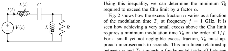
Summary. The manuscript considers a Chu-type electrically small antenna (TM01 mode, RLC model) with a series time-varying inductor L(t)=L0(1+h(t)) and asks which modulation waveform h(t) best violates the Chu Q lower bound. The authors define an instantaneous Q(t)=ωW_stored/P_total in which the modulator's work appears as an effective "modulation resistance" R_mod=L0 h'(t) in the dissipation denominator (Eqs. (13)–(15)). They then (i) analyze sinusoidal modulation and derive a trade-off between Q-excess α and modulation period T0 (Eqs. (4)–(7), Fig. 2); (ii) derive an Euler–Lagrange condition (24) for smooth h; (iii) state Lemma 2, that the functional J[h]=∫(Q−Q_Chu)dt is maximized by piecewise-constant (bang-bang) h with switches synchronized to I(t)=0; and (iv) derive an upper bound on switch transition time τ_sw in terms of antenna size, isolation/BER, and carrier frequency (Eqs. (31)–(34), Fig. 3), concluding that smaller antennas permit slower switches. The headline claim is that bang-bang switching is a "mathematical necessity" for breaking the Chu limit.

Significance. The problem is well motivated: waveform optimization for time-modulated matching networks is a genuinely open and useful question, and the circuit-level derivation showing that dL/dt enters the power balance as an effective resistance R_mod=L0h' (Eqs. (11)–(15)) is a concrete, self-contained modeling contribution. The paper fits no parameters to data and its claims are in principle checkable from its own equations, which is a strength. The §VI bound relating switch speed, electrical size, and BPSK error rate, while algebraically elementary, is the kind of design relation practitioners could use. However, the central optimality claim (Lemma 2) is not merely under-proved: as detailed below, the paper's own equations imply that the proposed bang-bang optimizer cannot satisfy the design constraint (4) it is meant to optimize, and the objective's sign convention is internally contradictory. If those issues were resolved the work could be a useful contribution, but the result as stated does not hold.

major comments (4)

[§II, §IV.B — Eqs. (4) and (17)] The optimization goal is internally contradictory. Eq. (4) (and (17)) require ∫ΔQ dt ≤ −αQ_Chu with α>0, i.e., Q driven *below* the Chu lower bound — the correct direction for 'breaking' the limit. Yet the text calls α a 'Q-factor excess', defines J in (17) as a functional 'to be maximized', and Lemma 2's proof argues the optimal profile 'achieves the maximum possible Q-factor'. Maximizing Q is the opposite of the stated constraint, and exceeding the Chu lower bound is trivial (it is a lower bound). The variational problem as actually solved in §IV–V is not the problem posed in §II. This sign/direction inconsistency propagates through the whole paper and must be resolved before any optimality statement can be evaluated.
[§V, Lemma 2 (with Eq. (15))] The proposed optimizer cannot meet its own constraint. In any constant segment of a piecewise-constant h, Eq. (15) gives Q=ω(La+L0(1+h))/(Ra+Rm). Since passivity requires h≥−1, Q≥ωLa/(Ra+Rm)=Q_Chu·Ra/(Ra+Rm): with Rm=0 this equals Q_Chu and never dips below it; with Rm>0 the dip is a static-loss effect unrelated to modulation. Hence ΔQ(t)≥0 a.e. and J≥0, so (4) fails for every α>0. The only term in the model capable of pushing Q below its static value is R_mod=L0h'>0 in D(h') — precisely the term Lemma 2 sets out to eliminate. The paper thus optimizes away the only mechanism that could achieve its objective. Conversely, if the intended goal is to *maximize* Q, the optimum is a constant h (no switching at all), which makes the bang-bang result vacuous. Either reading undermines the central claim.
[§III — Eqs. (6)–(7), Fig. 2] For the sinusoidal law L(t)=L0(1+cos ω_M t)≥0, Eq. (6) gives ΔQ=ωL(t)/R≥0, so the left side of (7), ω_M T0+sin(ω_M T0), is nonnegative on the relevant range and (7) is unsatisfiable for any α>0. Fig. 2 nevertheless plots positive α versus T0, which can only have been produced with a flipped sign convention. Additionally, (6) omits the modulation resistance R_mod that §IV derives as the essential effect (Eq. (15)), so the sinusoidal section and the variational section use different Q models. The figure and the underlying inequality need to be recomputed under a single, consistent sign convention and Q model.
[§IV.B–§V — Eq. (24) and Lemma 2 proof] There is no logical bridge from the Euler–Lagrange analysis to bang-bang optimality. Eq. (24) is a necessary condition only for C¹ extremals; constant segments (h'=h''=0) do not satisfy it (they would require ((Ra+Rm)/L0)²=0), so the claimed optimum lies outside the class for which the condition was derived, and no argument (e.g., Pontryagin-type analysis with h' as a bounded control, or a convexity/Lemma-1-based bound) is given to show the extremum over the enlarged class is piecewise constant. Lemma 2's proof is instead a verbal argument whose key premise — that transitions at I(t)=0 nullify the switching cost — does not address the denominator of (15) during the segments, and whose conclusion ('maximum possible Q-factor') contradicts (4) as noted above. As stated, Lemma 2 is unsupported.

minor comments (6)

[§IV.A, Lemma 1] The proof substitutes the average h0=(1/T0)∫h dt for h(t) in the numerator of Q, but the average of the ratio N(h)/D(h') is not bounded by the ratio evaluated at the average numerator; the step is not justified. Also the inequality directions involving Rlwr/Rupp need care given that Rlwr (a lower bound on L0h') can be negative. The lemma is not load-bearing for the main claim, but as stated its proof is incomplete.
[§IV.B, Eq. (17)] Writing the constraint '≤ −αQ_Chu' inside the definition of a functional that is then 'to be maximized' conflates the objective and the constraint; please separate J[h]:=∫(Q−Q_Chu)dt from the design inequality.
[§V, Lemma 2 proof] Undefined notation: 'transition velocity f′' and 'the derivative f′' — f is never defined; presumably h is meant. Also 'bypassing the inherent efficiency of smooth modulation functions' presumably should read 'inefficiency'.
[§VI, Eqs. (31)–(32)] The substitution Q=1/(kρ)³ uses the Chu *lower* bound as the operating Q in τ_ant, which yields the shortest natural decay and hence the most permissive τ_sw bound; this best-case character should be stated explicitly. Relatedly, the abstract's 'switching time becomes longer as antennas become electrically smaller' should read that the *upper bound on the allowable* switching time increases.
[Figures] Fig. 2 lacks axis labels and units (T0 axis presumably seconds; is the vertical axis α?). Fig. 3's heatmap has tick labels like −12…−7 with no stated quantity or colorbar (presumably log10(τ_sw) in seconds); axes (ρ/λ, Pe) should be labeled.
[General] Typos: 'instantananeous' (Lemma 1); 'from to which' (after (33)); integral lower limit 'ta' in Lemma 1's proof; inconsistent h vs f notation in §V. Eq. (22b) would benefit from an explicit intermediate step, as the algebra into (23)–(24) is easy to mis-check.

Circularity Check

0 steps flagged

No significant circularity: the variational and bang-bang claims are self-contained (if internally inconsistent) circuit-model arguments, not fits or self-citation loops.

full rationale

The paper builds Q(t,h) from a Chu RLC model plus a time-varying inductor (eqs. 1–15), applies a standard Euler–Lagrange argument to obtain the nonlinear ODE (24), then argues informally that piecewise-constant h nullifies Rmod (Lemma 2). The switching-time bound (31)–(34) is ordinary textbook decay plus the BPSK Pe formula. None of these steps redefine the target as an input, fit a parameter and relabel it a prediction, or rest the central claim on an unverified self-citation or author-imported uniqueness theorem. Citations are external (Chu, Alù, Grbic, Tretyakov, Pozar, Proakis). Internal sign/objective contradictions (ΔQ cannot go negative under the proposed optimizer; constants fail (24); sinusoidal section uses a different Q formula) are correctness failures, not circular reductions. Score 0 is therefore appropriate.

Axiom & Free-Parameter Ledger

3 free parameters · 6 axioms · 0 invented entities

The paper rests on the classical Chu RLC equivalent for a single TM01 ESA, a particular decomposition of instantaneous Q that folds modulator work into Ptotal as Rmod=L0 h', Lipschitz/power-nonnegativity restrictions for the Q bounds, a calculus-of-variations setup that assumes smooth competitors before concluding the optimum lies outside that class, and standard resonator ring-down plus BPSK Pe–SNR inversion for the switching bound. No numerical free parameters are fitted to measurements; β and S (or Pe) are designer-chosen thresholds. No new physical entity is postulated.

free parameters (3)

β (fractional occupancy of symbol period allowed for switching) = 0.25 in Fig. 3
Hand-chosen duty-cycle fraction in (30)–(34); Fig. 3 uses β=0.25 with no derivation that this value is optimal or necessary.
Isolation requirement S (or target Pe)
Designer threshold converting ring-down to an allowable switch window; enters (28)–(34) and the heatmap. Not fitted to data but freely set.
Rm (modulator internal loss resistance)
Appears in Reff and in the EL equation; left symbolic with no measured or derived value, yet it shifts both the Q bounds and the ODE coefficients.

axioms (6)

domain assumption Chu ESA equivalent circuit: single TM01 mode with C=ρ/(cR), L=ρR/c and QChu=ωLa/Ra (and later QChu=1/(kρ)^3).
Invoked in §II and again when substituting Q=1/(kρ)^3 into the switch-time bound (32).
ad hoc to paper Instantaneous Q(t)=ω Wstored(t)/Ptotal(t) with Ptotal including modulator work Pmod=I² dL/dt, yielding Rmod=L0 h' in the denominator.
Central modeling choice in (8)–(15). Standard cycle-averaged Q does not automatically include this term; the paper’s optimality argument stands or falls with this definition.
domain assumption Modulation h is Lipschitz with Rlwr ≤ L0 h' ≤ Rupp and does not produce negative instantaneous power (Lemma 1).
Used to bound average Q; rules out large negative Rmod that would otherwise drive Q through infinity or negative.
standard math Calculus of variations / Euler–Lagrange necessary condition applies to smooth competitors η with η(0)=η(T0)=0, producing the inductive modulation ODE (24).
§IV.B; standard EL machinery, applied to a functional whose optimum is later claimed to lie outside C¹.
ad hoc to paper Switching cost is nullified if transitions occur when I(t)=0, allowing ideal bang-bang without Rmod penalty (Lemma 2 proof).
Key step that lets piecewise-constant h evade the dissipation penalty; stated without a full impulse-control or measure-theoretic justification.
domain assumption Field ring-down A(t)=A0 e^{-t/τant} with τant=Q/(π fc), and BPSK Pe ↔ isolation S via S=10 log10[(1/2)(Qinv(Pe))²].
§VI and refs. [12],[13]; standard resonator and digital-comms formulas used to get (34).

reviewed 2026-07-30 · how reviews work

0 comments

Cite this review

Pith. "Pith review of Optimality of Bang-Bang Switching for Breaking the Chu Limit via Time-Modulated Matching." pith.science (2026). https://pith.science/paper/PXIQL4CP

@misc{pith2026260723688,
  author       = {Pith},
  title        = {Pith review of: Optimality of Bang-Bang Switching for Breaking the Chu Limit via Time-Modulated Matching},
  year         = {2026},
  howpublished = {\url{https://pith.science/paper/PXIQL4CP}},
  note         = {Machine review of arXiv:2607.23688}
}

Share X Bluesky LinkedIn Reddit HN

abstract

This paper shows that surpassing the Chu limit on $Q$-factors via time-modulated matching requires non-smooth switching strategies. We derive a nonlinear differential condition to show that differentiable modulation functions are sub-optimal, then show that the optimal switching trajectory for maximizing the violation of the Chu limit is a piecewise-constant (Bang-Bang) profile. Finally, we establish an upper-bound connecting the antenna size, switching speed, and bit error rate, which reveals that switching time becomes longer as antennas become electrically smaller.

Figures

Figures reproduced from arXiv: 2607.23688 by Miguel Rodrigo Castellanos, Mohamed Akrout.

**Figure 2.** Figure 2: shows how the excess fraction α varies as a function of the modulation time T0 at frequency f = 1 GHz. It is seen how achieving a very small excess above the Chu limit requires a minimum modulation time T0 on the order of 1/f. For a small yet not negligible excess fraction, T0 must approach microseconds to seconds. This non-linear relationship between α and T0 suggests a fundamental trade-off between the … view at source ↗

**Figure 3.** Figure 3: Heatmap of the maximum allowable switch transition t [PITH_FULL_IMAGE:figures/full_fig_p005_3.png] view at source ↗

discussion (0)

Reference graph

Works this paper leans on

13 extracted references

[1]

PCS antenna design: The challenge of miniaturization,

A. K. Skrivervik, J.-F. Zurcher, O. Staub, and J. Mosig, “ PCS antenna design: The challenge of miniaturization,” IEEE Antennas Propag. Mag , vol. 43, no. 4, pp. 12–27, 2002

2002
[2]

Physical limitations of omni-directional an tennas,

L. J. Chu, “Physical limitations of omni-directional an tennas,” J. Appl. Phys., vol. 19, no. 12, pp. 1163–1175, 1948

1948
[3]

Beyond Chu’s limit with Flo quet impedance matching,

H. Li, A. Mekawy, and A. Al` u, “Beyond Chu’s limit with Flo quet impedance matching,” Phys. Rev. Lett. , vol. 123, p. 164102, Oct 2019

2019
[4]

Space–ti me modu- lation of a multimode electrically small antenna for increa sed matching and efﬁciency bandwidths,

Z. Fritts, A. Babaee, S. M. Y oung, and A. Grbic, “Space–ti me modu- lation of a multimode electrically small antenna for increa sed matching and efﬁciency bandwidths,” IEEE Trans. Antennas Propag. , vol. 73, no. 3, pp. 1308–1320, Mar. 2025

2025
[5]

Antenna bandwidth engineering through time -varying resistance,

M. Mostafa, N. Ha-V an, P . Jayathurathnage, X. Wang, G. Pt itcyn, and S. Tretyakov, “Antenna bandwidth engineering through time -varying resistance,” Applied Physics Letters , vol. 122, no. 17, 2023

2023
[6]

UHF electrically small box cage loop antenna with an embedded no n-Foster load,

J. Church, J.-C. S. Chieh, L. Xu, J. D. Rockway, and D. Arce o, “UHF electrically small box cage loop antenna with an embedded no n-Foster load,” IEEE Antennas Wireless Propag. Lett. , vol. 13, pp. 1329–1332, Jul. 2014

2014
[7]

Broadband parametric im pedance matching for small antennas using the Bode-Fano limit: Impr oving on Chu’s limit for loaded small antennas,

P . Loghmannia and M. Manteghi, “Broadband parametric im pedance matching for small antennas using the Bode-Fano limit: Impr oving on Chu’s limit for loaded small antennas,” IEEE Antennas Propag. Mag. , vol. 64, no. 5, pp. 55–68, Oct 2022

2022
[8]

An energy-synchrono us direct antenna modulation method for phase shift keying,

K. Schab, D. Huang, and J. J. Adams, “An energy-synchrono us direct antenna modulation method for phase shift keying,” IEEE Open J. Antennas Propag., vol. 1, pp. 41–46, 2020

2020
[9]

A novel continuous direct antenna modulatio n system through varactor diode tuning,

I. M. Broadbooks, M. C. Smith, R. M. Radhakrishnan, and D. F. Sievenpiper, “A novel continuous direct antenna modulatio n system through varactor diode tuning,” IEEE Trans. Antennas Propag. , vol. 73, no. 4, pp. 2416–2426, Apr. 2025

2025
[10]

Parametric enhan cement of radiation from electrically small antennas,

A. Mekawy, H. Li, Y . Radi, and A. Al` u, “Parametric enhan cement of radiation from electrically small antennas,” Phys. Rev. Appl. , vol. 15, p. 054063, May 2021

2021
[11]

Time-varying components for enhancing wi reless transfer of power and information,

P . Jayathurathnage, F. Liu, M. S. Mirmoosa, X. Wang, R. F leury, and S. A. Tretyakov, “Time-varying components for enhancing wi reless transfer of power and information,” Phys. Rev. Appl., vol. 16, p. 014017, Jul 2021

2021
[12]

D. M. Pozar, Microwave engineering. John wiley & sons, 2011

2011
[13]

J. G. Proakis and M. Salehi, Digital communications . McGraw-hill New Y ork, 2001, vol. 4

2001

This paper was first reviewed by grok-4.5 on July 30, 2026.

[1] [1]

PCS antenna design: The challenge of miniaturization,

A. K. Skrivervik, J.-F. Zurcher, O. Staub, and J. Mosig, “ PCS antenna design: The challenge of miniaturization,” IEEE Antennas Propag. Mag , vol. 43, no. 4, pp. 12–27, 2002

2002

[2] [2]

Physical limitations of omni-directional an tennas,

L. J. Chu, “Physical limitations of omni-directional an tennas,” J. Appl. Phys., vol. 19, no. 12, pp. 1163–1175, 1948

1948

[3] [3]

Beyond Chu’s limit with Flo quet impedance matching,

H. Li, A. Mekawy, and A. Al` u, “Beyond Chu’s limit with Flo quet impedance matching,” Phys. Rev. Lett. , vol. 123, p. 164102, Oct 2019

2019

[4] [4]

Space–ti me modu- lation of a multimode electrically small antenna for increa sed matching and efﬁciency bandwidths,

Z. Fritts, A. Babaee, S. M. Y oung, and A. Grbic, “Space–ti me modu- lation of a multimode electrically small antenna for increa sed matching and efﬁciency bandwidths,” IEEE Trans. Antennas Propag. , vol. 73, no. 3, pp. 1308–1320, Mar. 2025

2025

[5] [5]

Antenna bandwidth engineering through time -varying resistance,

M. Mostafa, N. Ha-V an, P . Jayathurathnage, X. Wang, G. Pt itcyn, and S. Tretyakov, “Antenna bandwidth engineering through time -varying resistance,” Applied Physics Letters , vol. 122, no. 17, 2023

2023

[6] [6]

UHF electrically small box cage loop antenna with an embedded no n-Foster load,

J. Church, J.-C. S. Chieh, L. Xu, J. D. Rockway, and D. Arce o, “UHF electrically small box cage loop antenna with an embedded no n-Foster load,” IEEE Antennas Wireless Propag. Lett. , vol. 13, pp. 1329–1332, Jul. 2014

2014

[7] [7]

Broadband parametric im pedance matching for small antennas using the Bode-Fano limit: Impr oving on Chu’s limit for loaded small antennas,

P . Loghmannia and M. Manteghi, “Broadband parametric im pedance matching for small antennas using the Bode-Fano limit: Impr oving on Chu’s limit for loaded small antennas,” IEEE Antennas Propag. Mag. , vol. 64, no. 5, pp. 55–68, Oct 2022

2022

[8] [8]

An energy-synchrono us direct antenna modulation method for phase shift keying,

K. Schab, D. Huang, and J. J. Adams, “An energy-synchrono us direct antenna modulation method for phase shift keying,” IEEE Open J. Antennas Propag., vol. 1, pp. 41–46, 2020

2020

[9] [9]

A novel continuous direct antenna modulatio n system through varactor diode tuning,

I. M. Broadbooks, M. C. Smith, R. M. Radhakrishnan, and D. F. Sievenpiper, “A novel continuous direct antenna modulatio n system through varactor diode tuning,” IEEE Trans. Antennas Propag. , vol. 73, no. 4, pp. 2416–2426, Apr. 2025

2025

[10] [10]

Parametric enhan cement of radiation from electrically small antennas,

A. Mekawy, H. Li, Y . Radi, and A. Al` u, “Parametric enhan cement of radiation from electrically small antennas,” Phys. Rev. Appl. , vol. 15, p. 054063, May 2021

2021

[11] [11]

Time-varying components for enhancing wi reless transfer of power and information,

P . Jayathurathnage, F. Liu, M. S. Mirmoosa, X. Wang, R. F leury, and S. A. Tretyakov, “Time-varying components for enhancing wi reless transfer of power and information,” Phys. Rev. Appl., vol. 16, p. 014017, Jul 2021

2021

[12] [12]

D. M. Pozar, Microwave engineering. John wiley & sons, 2011

2011

[13] [13]

J. G. Proakis and M. Salehi, Digital communications . McGraw-hill New Y ork, 2001, vol. 4

2001

Optimality of Bang-Bang Switching for Breaking the Chu Limit via Time-Modulated Matching

The reading

Core claim §

What carries the argument

Load-bearing premise §

What would settle it §

If this is right

Where Pith is reading between the lines

discussion (0)

Core claim

Load-bearing premise

What would settle it