REVIEW 4 major objections 8 minor 64 references
A Multi-stage Constrained Optimization Framework for Data-driven Problems
T0 review · 4 major / 8 minor · reviewed 2026-07-30 · grok-4.5
Pith's one-line read A multi-stage VAE framework turns noisy data-driven problems into low-dimensional surrogates and solves them with hard constraint priority, recovering analytic optima and novel feasible molecules.
desk verdict Workable staged VAE+filter recipe with clean synthetic ablations; the ZINC “0% violation” claim does not line up with the paper’s own ε_v and reactivity numbers. read the letter →
The pith
A machine-rendered reading of the paper's core claim, the machinery that carries it, and where it could break.
The reading
What carries the argument
The constraint-priority filter method (CPFM): it reframes the latent surrogate as the bi-objective pair (objective, violation), always prefers a violation-reduction step until feasibility tolerance is met, then accepts candidate steps only when they are not dominated under a filter envelope, thereby guaranteeing surrogate feasibility without estimating Lagrange multipliers.
What would settle it
Recompute the drug-design molecules with an independent external calculator for reactivity and logP; if a non-negligible fraction violate the stated bounds, the hard-constraint claim fails for that task.
Extended reading notes
Core claim
MCOF returns solutions that are feasible for the learned Stage-2 surrogate to a stated tolerance and near-optimal on the surrogate objective; on a synthetic constrained problem it recovers the analytic optimum, and on a ZINC250k molecular-weight / logP / reactivity task it yields 0 % constraint violations and 100 % novel molecules.
Load-bearing premise
That a point declared feasible by the learned neural surrogate is close enough to true black-box feasibility for the claim of hard constraints to hold.
Editorial extensions
If this is right
- Latent-space optimization can enforce hard feasibility by filter methods instead of unstable multiplier search.
- Embedding targets only into low-entropy latent coordinates leaves the remaining dimensions free for diversity sampling after a single optimized solution is found.
- Uniformizing the aggregate posterior removes Gaussian-mixture wrinkles that otherwise destroy convexity of the surrogate landscape.
- The same staged pipeline applies unchanged to both continuous synthetic problems and mixed-integer SMILES-based molecular design.
Reading between the lines
- If the surrogate-to-true gap remains small across domains, MCOF could replace post-hoc repair steps that currently dominate constrained generative design.
- The entropy-floor plus feature-selector combination offers an automatic, less inductive-bias-prone route to the kind of disentanglement that is usually inspected by hand.
- Extending CPFM’s filter to true multi-objective fronts (rather than a single objective plus violation) is a direct next experiment the architecture already supports.
Editorial analysis
A structured set of objections, weighed in public.
Referee Report
Summary. The paper proposes MCOF, a four-stage pipeline for data-driven constrained optimization in VAE latent spaces: (1) an entropy-constrained VAE (EC-VAE) with a one-sided aggregate-posterior entropy floor, coupled to an entropy-ordered feature selector that embeds objective/constraint targets into low-entropy latent dimensions; (2) a Uniform Transformation (UT) module (G-KDE → Gaussian-mixture fit → probability integral transform) mapping the aggregate posterior to a uniform box, with a retrained decoder and MLP surrogate regressor; (3) a constraint-priority filter method (CPFM) that alternates violation-reduction and objective-reduction trust-region steps under a Fletcher–Leyffer-style filter acceptance test on the surrogate; and (4) resampling of unselected latent coordinates for solution diversity. Validation comprises a synthetic 10-D problem with known analytic optimum (recovered: y*=32, Table II) with per-stage ablations (Figs. 6–10, Tables I–IV), and a ZINC250k molecular task minimizing molecular weight subject to logP ∈ [1,3] and zero reactivity, where the authors report 0% constraint violation and 100% novelty (Table V).
Significance. If the feasibility claims hold, the paper offers a genuinely modular and reasonably well-motivated framework: the aggregate- vs conditional-posterior entropy discussion around Eq. (3)–(4) is careful and correct, the synthetic study recovers the analytic optimum and ablates each stage separately (the strongest evidence in the paper), and CPFM is a sensible, multiplier-free adaptation of classical filter methods to neural surrogates with an explicit feasibility tolerance. The synthetic ablations (UT manifold smoothing in Fig. 9, CPFM vs. penalty in Fig. 10) are the kind of stage-wise evidence rarely provided in this subarea. However, the headline real-world claim — "hard constraint" satisfaction with 0% violation on the drug task — currently rests on an internally inconsistent tolerance accounting and on a self-certified constraint (reactivity scored by the same regressor used inside the optimizer), which substantially limits the significance as written. The contribution is incremental over the authors' prior UT module [53] but the integration and the CPFM stage are new enough to merit publication once the feasibility reporting is repaired.
major comments (4)
- [§IV-D/§IV-E, Eq. (17), Tables V–VI; also Table II] The reported results are inconsistent with the stated feasibility tolerance, and the equality constraint is self-certified. §IV-A sets ε_v = 1e-5 and §IV-D states the same tolerances are used for the drug task. Under Eq. (17), CPFM's return condition (Alg. 3, lines 14 and 23) certifies v(ζ*) ≤ 1e-5, which — given logP inside [1,3] — requires |reactivity| ≲ √ε_v ≈ 3.2e-3 in the optimizer's units. Yet Table VI reports reactivity −0.024, −0.011, −0.009 and Table V a mean of −0.013; squared, these contribute 8e-5 to 5.8e-4 to v, one to two orders of magnitude above ε_v. The same issue appears in miniature in the synthetic case: Table II's 'Estimation' row gives ĉ_E = −4.4e-3, i.e. v ≈ 1.9e-5 > ε_v at the returned point. Either the tables are in denormalized units while the tolerance is in normalized units (nowhere stated — and the raw scale of 'reactivity' is never defined, nor is it said ho
- [§IV-E, Table V] The head-to-head comparison in Table V does not support the superiority framing in the text. Most baseline cells are missing ('–'), and the baselines demonstrably solved different problems: MolDQN's logP of 11.84 versus MCOF's 2.98 reflects that MCOF was constrained to [1,3] by construction, not that it optimizes better; likewise MCOF's QED (0.58) is worse than VAE+GA (0.75) and MolDQN (0.859), which the text does not acknowledge. The paragraph below the table should be rewritten to state explicitly that the comparison is across methods solving heterogeneous tasks, and the claims limited to what the table shows (constraint enforcement and novelty under MCOF's own formulation). Two further reporting gaps: the text says 'We generated 10 candidate solutions' but Table VI is drawn from 'the 100 generated samples' — which is it, and what is the denominator of the 0% violation rate? And SMILES
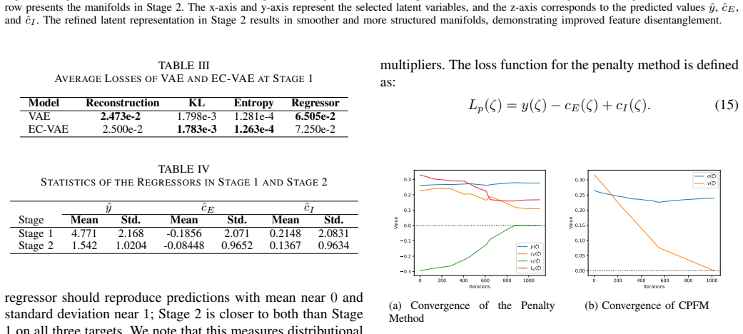
- [§IV-C3, Eq. (15); Abstract] The abstract and §II-B claim CPFM 'demonstrably improves feasibility relative to standard penalty or Lagrangian-based approaches,' but the only comparison (Fig. 10) is against a single fixed linear penalty L_p = y − c_E + c_I with unit weights (Eq. 15). The sign pattern (why −c_E for an equality constraint rather than |c_E| or c_E²?) is unmotivated, unit weights are a known-bad setting for exactly the reason shown, and no tuned-penalty or augmented-Lagrangian baseline is tried. As written this is a strawman for the comparative claim. Either add a penalty-parameter sweep and/or an augmented Lagrangian baseline on the synthetic problem, or narrow the claim to what Fig. 10 shows (an unweighted linear penalty fails to satisfy the equality constraint; CPFM does not).
- [§IV-E (feature selector outcome); §III-B narrative] In the drug task the feature selector retained 252 of 256 latent dimensions. This is in tension with the framework's central narrative — that Stage 1 concentrates targets into a small low-entropy subset so that optimization proceeds 'over a low-dimensional subspace' (Abstract) — and with Stage 4's role of resampling unselected coordinates for diversity (here only 4 dimensions). The remark that this 'limit[s] the number of feasible solutions' is unexplained: why would a large selected set limit feasible-solution count rather than diversity? Please report the entropy spectrum and the selector trajectory (α, s over epochs) for the drug task, state which targets actually live in which dimensions, and discuss whether Stage 1 is functioning as designed on this problem or effectively inactive.
minor comments (8)
- [Fig. 9] Panel captions (b) and (c) appear swapped relative to their z-axis labels: (b) is captioned ĉ_E but its axis reads c_I, and vice versa for (c); same for (e)/(f). Please check and correct.
- [§IV-C2, Table IV] Table IV is described as showing a 'well-calibrated regressor' because predictions have mean ≈ 0 and std ≈ 1 after normalization; the text concedes this 'measures distributional calibration rather than predictive accuracy.' Since moment matching is neither calibration nor accuracy, please report held-out RMSE/R² per target for the Stage-1 and Stage-2 regressors instead (or in addition); the 57%/89% loss reductions quoted in the same paragraph are the more meaningful numbers.
- [§IV-C1, Table III] Table III shows the vanilla VAE's regressor loss (6.505e-2) is slightly better than EC-VAE's (7.250e-2), which the text acknowledges but does not discuss. Since Stage 1's purpose is to make the targets regressible from the selected subset, please explain why the EC-VAE trade-off (worse raw regression, better disentanglement per Figs. 6–8) is the right one for the downstream optimization.
- [§IV-E] Please define 'reactivity' operationally: what property of a ZINC molecule is it, how were the training labels computed, and in what units? Also state how logP and MWt were evaluated for generated molecules (e.g., RDKit) and confirm these two were computed externally rather than from the surrogate.
- [Eq. (15)] Clarify the sign choice L_p = y(ζ) − c_E(ζ) + c_I(ζ): for an equality constraint this rewards driving c_E negative without bound, which differs from any standard penalty. If this is a typo for +|c_E| or c_E², correct it; if intentional, justify it.
- [Notation (global)] (i) 'V AE' with a spurious space appears throughout (presumably a typesetting artifact). (ii) γ is used both as the entropy-floor weight in Eq. (3) and, as γ_v, γ_o, for the filter envelope in Alg. 3; consider renaming one. (iii) In Eq. (12) and (17), state explicitly that max acts elementwise and the norms reduce to scalars (the text does this for (12) but not where (17) is introduced).
- [Reproducibility] No code or data availability statement is given. Given that the paper's evidential weight rests on numerical ablations, releasing the synthetic-problem code and the trained surrogate/CPFM configuration (all CPFM hyperparameters ε_v, ε_o, γ_v, γ_o, Δ_0, Δ_min, τ, K, N_max are currently unspecified numerically except ε_v = ε_o = 1e-5) would materially strengthen the paper.
- [§IV-B, Table I] Table I shows x4–x10 have standard deviations of 23–67 (essentially the U(−50,50) sampling range), confirming they are irrelevant dimensions; a one-line remark connecting this to the problem structure (only x1–x3 appear in Eq. (14)) would help readers parse the table.
Circularity Check
No load-bearing circular derivation; only mild self-evaluation of surrogate feasibility on the drug task (reactivity/Vio scored by the same regressor CPFM optimizes).
-
fitted input called prediction
[§III-D Eq. (12)/(17); Alg. 3; §IV-E Table V]
"We emphasize that v is built from the learned regressor P_ψ̃, so the feasibility CPFM certifies is feasibility with respect to the surrogate. ... Reactivity (Reac.) is reported from the Stage 2 MLP regressor rather than a direct calculation, as a suitable external measure is unavailable. ... MCOF (ours) ... Reac. -0.013 ... Vio. 0%"
CPFM’s return condition requires v(ζ*)≤ε_v with v defined from the same Stage-2 MLP that supplies the reported reactivity and the Vio.=0% column. On the drug task, “0% violation” therefore largely restates that CPFM terminated under its own surrogate acceptance test, not an independent external feasibility measurement. (Synthetic Table II does use true decoded constraints; the circularity is confined to the drug reactivity/Vio reporting.)
full rationale
MCOF is an engineering pipeline (EC-VAE + feature selector, UT, CPFM, latent completion), not a first-principles derivation that equates a claimed prediction to its fitted inputs by algebra. The synthetic case recovers the known analytic optimum and reports independent validation statistics computed from decoded x (Table II), which is ordinary empirical check rather than circularity. Self-citation of the author’s prior UT module [53] is component reuse, not a uniqueness theorem or load-bearing premise that forces the main claims. The sole mild circularity-adjacent pattern is on ZINC: CPFM is defined to return points with v(ζ)≤ε_v where v is built from the Stage-2 regressor P_ψ̃ (§III-D, Eq. 12/17, Alg. 3), and Table V’s Reac./Vio.=0% are taken from that same regressor because “a suitable external measure is unavailable” (§IV-E). Reporting surrogate feasibility after a successful CPFM run partly restates the optimizer’s own acceptance test. The paper explicitly frames the certificate as surrogate feasibility and notes the true-constraint gap, so this is evaluation design weakness rather than a closed self-definitional loop; score 2, not higher.
Assumptions & free parameters
free parameters (8)
- β (KL weight in L_EC) =
6 (synthetic); 0.3 (ZINC)
- γ (entropy-bound weight) =
1
- η (per-dimension entropy floor) =
≈1.42
- λ (regressor vs EC-VAE loss weight)
- α, ρ, s_min, T (feature-selector schedule)
- ε_v, ε_o, γ_v, γ_o, Δ_0, Δ_min, τ, K, N_max (CPFM) =
ε_v=ε_o=1e-5 (reported); others partially unspecified
- UT output box [-4,4] and G-KDE bandwidth (Scott) =
[-4,4]; Scott h=n^{-1/5}σ
- Network widths / latent sizes =
l=10 / l=256 as stated
assumptions (6)
- standard math Standard VAE ELBO / reparameterization and Gaussian prior structure (Fig. 1, Eq. 3 first two terms).
- standard math Probability integral transform maps a continuous CDF to Uniform(0,1) coordinatewise (Stage 2.3, Eq. 9).
- domain assumption Classic filter acceptance with sufficient-reduction envelopes yields progress toward feasible descent (Alg. 3; cite Fletcher et al.).
- ad hoc to paper Lower-entropy aggregate-posterior dimensions are the right place to embed objective/constraint targets, while high-entropy dims carry data identity (§III-B, Alg. 1).
- domain assumption Surrogate feasibility of P_ψ̃ within tolerance implies useful true feasibility up to surrogate error (§III-D).
- domain assumption G-KDE modes identify a faithful finite Gaussian mixture for each latent margin (Alg. 2).
invented entities (4)
-
EC-VAE (entropy-constrained VAE with one-sided entropy floor on aggregate posteriors)
-
Uniform Transformation (UT) module as staged G-KDE → GM → PIT pipeline
-
Constraint-priority filter method (CPFM)
-
Latent feature selector mask w with entropy-ordered geometric shrinking
Cite this review
Pith. "Pith review of A Multi-stage Constrained Optimization Framework for Data-driven Problems." pith.science (2026). https://pith.science/paper/QHFUDHZA
@misc{pith2026260723480,
  author       = {Pith},
  title        = {Pith review of: A Multi-stage Constrained Optimization Framework for Data-driven Problems},
  year         = {2026},
  howpublished = {\url{https://pith.science/paper/QHFUDHZA}},
  note         = {Machine review of arXiv:2607.23480}
}
read the original abstract
Variational autoencoders (VAEs) transform high-dimensional, often noisy data into a compact latent representation, making downstream optimization more tractable. Three challenges persist in VAE-based constrained optimization: (i) sampling effectively within the latent space, (ii) identifying the active decision variables that actually influence the objective and constraints, and (iii) enforcing constraints without destabilizing training. We propose a Multi-stage Constrained Optimization Framework (MCOF). First, an entropy-constrained VAE (EC-VAE) coupled with a feature selector embeds objective and constraint information into a designated subset of latent variables, so that optimization proceeds over a low-dimensional subspace while the remaining coordinates supply solution diversity. Second, a Uniform Transformation (UT) module applies a per-dimension probability integral transform, replacing the irregular aggregate posterior with a uniform distribution over a bounded box and mitigating posterior collapse and Gaussian mixture bias. Third, a constraint-priority filter method (CPFM) solves the resulting surrogate problem by alternating violation-reduction and objective-reduction steps under a filter acceptance test, returning solutions that are feasible for the learned surrogate to a specified tolerance without requiring multiplier estimation. Finally, unselected latent coordinates are resampled to generate diverse decodings of a single optimized solution. We validate MCOF on a synthetic problem, where we ablate each stage and recover the analytic optimum, and on a ZINC250k drug design task, where the generated molecules satisfy the imposed constraints and are entirely novel relative to the training set.
Figures


Figures from the paper (7 more)


Reference graph
Works this paper leans on
-
[53]
Uniform Transformation: Refining Latent Representation in Variational Autoencoders,
Y . Shi and C. S. George Lee, “Uniform Transformation: Refining Latent Representation in Variational Autoencoders,” in2024 IEEE 20th Inter- national Conference on Automation Science and Engineering (CASE), Aug. 2024, pp. 2786–2792
2024
-
[1]
An Introduction to Variational Autoen- coders,
D. P. Kingma and M. Welling, “An Introduction to Variational Autoen- coders,”Foundations and Trends® in Machine Learning, vol. 12, no. 4, pp. 307–392, Nov. 2019
2019
-
[2]
Shape your Space: A Gaussian Mixture Regularization Approach to Deterministic Autoencoders,
A. Saseendran, K. Skubch, S. Falkner, and M. Keuper, “Shape your Space: A Gaussian Mixture Regularization Approach to Deterministic Autoencoders,” inAdvances in Neural Information Processing Systems, vol. 34. Curran Associates, Inc., 2021, pp. 7319–7332
2021
-
[3]
Machine learning framework for quantum sampling of highly constrained, continuous optimization problems,
B. A. Wilson, Z. A. Kudyshev, A. V . Kildishev, S. Kais, V . M. Shalaev, and A. Boltasseva, “Machine learning framework for quantum sampling of highly constrained, continuous optimization problems,” Applied Physics Reviews, vol. 8, no. 4, p. 041418, Dec. 2021
2021
-
[4]
COIL: Constrained optimization in learned latent space: Learning representations for valid solutions,
P. J. Bentley, S. L. Lim, A. Gaier, and L. Tran, “COIL: Constrained optimization in learned latent space: Learning representations for valid solutions,” inProceedings of the Genetic and Evolutionary Computation Conference Companion, ser. GECCO ’22. New York, NY , USA: Association for Computing Machinery, Jul. 2022, pp. 1870–1877
2022
-
[5]
Constrained Bayesian Optimization for Automatic Chemical Design,
R.-R. Griffiths and J. M. Hern ´andez-Lobato, “Constrained Bayesian Optimization for Automatic Chemical Design,” Aug. 2019
2019
-
[6]
Learning Heuristics for Combinatorial Optimization Prob- lems with Deep Neural Networks,
A. Hottung, “Learning Heuristics for Combinatorial Optimization Prob- lems with Deep Neural Networks,” Ph.D. dissertation, Bielefeld Univer- sity, Jan. 2023
2023
-
[7]
Improving black- box optimization in V AE latent space using decoder uncertainty,
P. Notin, J. M. Hern ´andez-Lobato, and Y . Gal, “Improving black- box optimization in V AE latent space using decoder uncertainty,” in Advances in Neural Information Processing Systems, vol. 34. Curran Associates, Inc., 2021, pp. 802–814
2021
Show all 64 references
-
[8]
Constrained Generation of Semantically Valid Graphs via Regularizing Variational Autoencoders,
T. Ma, J. Chen, and C. Xiao, “Constrained Generation of Semantically Valid Graphs via Regularizing Variational Autoencoders,” inAdvances in Neural Information Processing Systems, vol. 31. Curran Associates, Inc., 2018
2018
-
[9]
Constrained Graph Variational Autoencoders for Molecule Design,
Q. Liu, M. Allamanis, M. Brockschmidt, and A. Gaunt, “Constrained Graph Variational Autoencoders for Molecule Design,” inAdvances in Neural Information Processing Systems, vol. 31. Curran Associates, Inc., 2018
2018
-
[10]
Automatic chemical design using a data-driven continuous representation of molecules,
R. G ´omez-Bombarelli, J. N. Wei, D. Duvenaud, J. M. Hern ´andez- Lobato, B. S ´anchez-Lengeling, D. Sheberla, J. Aguilera-Iparraguirre, T. D. Hirzel, R. P. Adams, and A. Aspuru-Guzik, “Automatic chemical design using a data-driven continuous representation of molecules,”ACS C...
2018
-
[11]
End-to-End Constrained Optimization Learning: A Survey,
J. Kotary, F. Fioretto, P. Van Hentenryck, and B. Wilder, “End-to-End Constrained Optimization Learning: A Survey,” inProceedings of the Thirtieth International Joint Conference on Artificial Intelligence. Mon- treal, Canada: International Joint Conferences on Artificial Intel...
2021
-
[12]
Diagnosing and Enhancing V AE Models,
B. Dai and D. Wipf, “Diagnosing and Enhancing V AE Models,” Oct. 2019
2019
-
[13]
Bayesian deep convolutional encoder–decoder networks for surrogate modeling and uncertainty quantification,
Y . Zhu and N. Zabaras, “Bayesian deep convolutional encoder–decoder networks for surrogate modeling and uncertainty quantification,”Journal of Computational Physics, vol. 366, pp. 415–447, Aug. 2018
2018
-
[14]
Variational Autoencoder-Based Metamodeling for Multi-Objective Topology Optimization of Electrical Machines,
V . Parekh, D. Flore, and S. Sch ¨ops, “Variational Autoencoder-Based Metamodeling for Multi-Objective Topology Optimization of Electrical Machines,”IEEE Transactions on Magnetics, vol. 58, no. 9, pp. 1–4, Sep. 2022
2022
-
[15]
Neural Architecture Optimization with Graph V AE,
J. Li, Y . Liu, J. Liu, and W. Wang, “Neural Architecture Optimization with Graph V AE,” Jun. 2020
2020
-
[16]
DC3: A learning method for optimization with hard constraints,
P. L. Donti, D. Rolnick, and J. Z. Kolter, “DC3: A learning method for optimization with hard constraints,”arXiv:2104.12225 [cs, math, stat], Apr. 2021
2021 arXiv
-
[17]
Lagrangian Duality for Constrained Deep Learning,
F. Fioretto, P. Van Hentenryck, T. W. K. Mak, C. Tran, F. Baldo, and M. Lombardi, “Lagrangian Duality for Constrained Deep Learning,” inMachine Learning and Knowledge Discovery in Databases. Applied Data Science and Demo Track, ser. Lecture Notes in Computer Science, 14 Y . Do...
2021
-
[18]
Self-Supervised Primal-Dual Learning for Constrained Optimization,
S. Park and P. V . Hentenryck, “Self-Supervised Primal-Dual Learning for Constrained Optimization,”Proceedings of the AAAI Conference on Artificial Intelligence, vol. 37, no. 4, pp. 4052–4060, Jun. 2023
2023
-
[19]
Loss landscapes and optimization in over-parameterized non-linear systems and neural networks,
C. Liu, L. Zhu, and M. Belkin, “Loss landscapes and optimization in over-parameterized non-linear systems and neural networks,”Applied and Computational Harmonic Analysis, vol. 59, pp. 85–116, Jul. 2022
2022
-
[20]
Optimizing Variational Graph Au- toencoder for Community Detection with Dual Optimization,
J. J. Choong, X. Liu, and T. Murata, “Optimizing Variational Graph Au- toencoder for Community Detection with Dual Optimization,”Entropy, vol. 22, no. 2, p. 197, Feb. 2020
2020
-
[21]
Pythae: Unifying Generative Autoencoders in Python – A Benchmarking Use Case,
C. Chadebec, L. J. Vincent, and S. Allassonni `ere, “Pythae: Unifying Generative Autoencoders in Python – A Benchmarking Use Case,” Jul. 2023
2023
-
[22]
Variational Inference with Normalizing Flows,
D. J. Rezende and S. Mohamed, “Variational Inference with Normalizing Flows,”arXiv:1505.05770 [cs, stat], Jun. 2016
2016 arXiv
-
[23]
Improving Variational Inference with Inverse Autoregres- sive Flow,
D. P. Kingma, T. Salimans, R. Jozefowicz, X. Chen, I. Sutskever, and M. Welling, “Improving Variational Inference with Inverse Autoregres- sive Flow,” Jan. 2017
2017
-
[24]
Improving Variational Auto-Encoders using Householder Flow,
J. M. Tomczak and M. Welling, “Improving Variational Auto-Encoders using Householder Flow,” Jan. 2017
2017
-
[25]
Importance Weighted Autoencoders,
Y . Burda, R. Grosse, and R. Salakhutdinov, “Importance Weighted Autoencoders,” Nov. 2016
2016
-
[26]
Posterior Collapse and Latent Variable Non-identifiability,
Y . Wang, D. Blei, and J. P. Cunningham, “Posterior Collapse and Latent Variable Non-identifiability,” inAdvances in Neural Information Processing Systems, vol. 34. Curran Associates, Inc., 2021, pp. 5443– 5455
2021
-
[27]
Disentangling by Factorising,
H. Kim and A. Mnih, “Disentangling by Factorising,” inInternational Conference on Machine Learning, Feb. 2018
2018
-
[28]
Isolating Sources of Disentanglement in Variational Autoencoders,
R. T. Q. Chen, X. Li, R. B. Grosse, and D. K. Duvenaud, “Isolating Sources of Disentanglement in Variational Autoencoders,” inAdvances in Neural Information Processing Systems, vol. 31. Curran Associates, Inc., 2018
2018
-
[29]
Deep Unsupervised Clustering with Gaussian Mixture Variational Autoencoders,
N. Dilokthanakul, P. A. M. Mediano, M. Garnelo, M. C. H. Lee, H. Salimbeni, K. Arulkumaran, and M. Shanahan, “Deep Unsupervised Clustering with Gaussian Mixture Variational Autoencoders,” Jan. 2017
2017
-
[30]
From Variational to Deterministic Autoencoders,
P. Ghosh, M. S. M. Sajjadi, A. Vergari, M. Black, and B. Sch ¨olkopf, “From Variational to Deterministic Autoencoders,” May 2020
2020
-
[31]
Improving Variational Encoder-Decoders in Dialogue Generation,
X. Shen, H. Su, S. Niu, and V . Demberg, “Improving Variational Encoder-Decoders in Dialogue Generation,” Feb. 2018
2018
-
[32]
Generative Models for Irregular Sequential Data,
S. Safar, “Generative Models for Irregular Sequential Data,” Master’s thesis, Aalto University, Aug. 2021
2021
-
[33]
Generative Modeling of Regular and Irregular Time Series Data via Koopman V AEs,
I. Naiman, N. B. Erichson, P. Ren, M. W. Mahoney, and O. Azencot, “Generative Modeling of Regular and Irregular Time Series Data via Koopman V AEs,” Oct. 2023
2023
-
[34]
AutoV AE: Mismatched Variational Autoencoder with Irregular Posterior-Prior Pairing,
T. Koike-Akino and Y . Wang, “AutoV AE: Mismatched Variational Autoencoder with Irregular Posterior-Prior Pairing,” in2022 IEEE International Symposium on Information Theory (ISIT), Jun. 2022, pp. 1689–1694
2022
-
[35]
Autoencoding Variational Autoencoder,
A. T. Cemgil, S. Ghaisas, K. Dvijotham, S. Gowal, and P. Kohli, “Autoencoding Variational Autoencoder,” Dec. 2020
2020
-
[36]
Coupled Variational Autoencoder,
X. Hao and P. Shafto, “Coupled Variational Autoencoder,” Jun. 2023
2023
-
[37]
Denoising Diffusion Probabilistic Models,
J. Ho, A. Jain, and P. Abbeel, “Denoising Diffusion Probabilistic Models,” Dec. 2020
2020
-
[38]
NV AE: A Deep Hierarchical Variational Autoencoder,
A. Vahdat and J. Kautz, “NV AE: A Deep Hierarchical Variational Autoencoder,” inAdvances in Neural Information Processing Systems, vol. 33. Curran Associates, Inc., 2020, pp. 19 667–19 679
2020
-
[39]
Challenging Common Assumptions in the Unsupervised Learning of Disentangled Representations,
F. Locatello, S. Bauer, M. Lucic, G. Raetsch, S. Gelly, B. Sch ¨olkopf, and O. Bachem, “Challenging Common Assumptions in the Unsupervised Learning of Disentangled Representations,” inProceedings of the 36th International Conference on Machine Learning. PMLR, May 2019, pp. 4114–4124
2019
-
[40]
Imposing Hard Constraints on Deep Networks: Promises and Limitations,
P. M ´arquez-Neila, M. Salzmann, and P. Fua, “Imposing Hard Constraints on Deep Networks: Promises and Limitations,”arXiv:1706.02025 [cs], Jun. 2017
2017 arXiv
-
[41]
A Primal Dual Formulation For Deep Learning With Constraints,
Y . Nandwani, A. Pathak, Mausam, and P. Singla, “A Primal Dual Formulation For Deep Learning With Constraints,” inAdvances in Neural Information Processing Systems, vol. 32. Curran Associates, Inc., 2019
2019
-
[42]
A Brief History of Filter Methods,
R. Fletcher, S. Leyffer, and P. L. Toint, “A Brief History of Filter Methods,” Oct. 2006. [Online]. Available: https://optimization-online. org/?p=10003
2006
-
[43]
The Statistical Filter Approach to Constrained Optimization,
T. Pourmohamad and H. K. H. Lee, “The Statistical Filter Approach to Constrained Optimization,”Technometrics, vol. 62, no. 3, pp. 303–312, Jul. 2020. [Online]. Available: https://www.tandfonline.com/doi/full/10. 1080/00401706.2019.1638304
2020
-
[44]
Deep learning methods for inverse problems,
S. Kamyab, Z. Azimifar, R. Sabzi, and P. Fieguth, “Deep learning methods for inverse problems,”PeerJ Computer Science, vol. 8, p. e951, May 2022
2022
-
[45]
Denoising criterion for variational auto-encoding framework,
D. J. Im, S. Ahn, R. Memisevic, and Y . Bengio, “Denoising criterion for variational auto-encoding framework,” inProceedings of the Thirty- First AAAI Conference on Artificial Intelligence, ser. AAAI’17. San Francisco, California, USA: AAAI Press, Feb. 2017, pp. 2059–2065
2017
-
[46]
Solving Bayesian Inverse Problems via Variational Autoencoders,
H. Goh, S. Sheriffdeen, J. Wittmer, and T. Bui-Thanh, “Solving Bayesian Inverse Problems via Variational Autoencoders,” Dec. 2021
2021
-
[47]
Variational Autoencoder Inverse Mapper: An End-to-End Deep Learning Framework for Inverse Problems,
M. Almaeen, Y . Alanazi, N. Sato, W. Melnitchouk, M. P. Kuchera, and Y . Li, “Variational Autoencoder Inverse Mapper: An End-to-End Deep Learning Framework for Inverse Problems,” in2021 International Joint Conference on Neural Networks (IJCNN), Jul. 2021, pp. 1–8
2021
-
[48]
Electric Machine Inverse Design with Variational Auto-Encoder (V AE),
Y . Xu, B. Wang, Y . Sakamoto, T. Yamamoto, Y . Nishimura, T. Koike- Akino, and Y . Wang, “Electric Machine Inverse Design with Variational Auto-Encoder (V AE),” in2023 IEEE Energy Conversion Congress and Exposition (ECCE), Oct. 2023, pp. 6338–6344
2023
-
[49]
Recent Advances in Adversarial Training for Adversarial Robustness,
T. Bai, J. Luo, J. Zhao, B. Wen, and Q. Wang, “Recent Advances in Adversarial Training for Adversarial Robustness,” inTwenty-Ninth International Joint Conference on Artificial Intelligence, vol. 5, Aug. 2021, pp. 4312–4321
2021
-
[50]
Inverse Optimization: Theory and Applications,
T. C. Y . Chan, R. Mahmood, and I. Y . Zhu, “Inverse Optimization: Theory and Applications,”Operations Research, Dec. 2023
2023
-
[51]
Intriguing properties of neural networks,
C. Szegedy, W. Zaremba, I. Sutskever, J. Bruna, D. Erhan, I. Goodfellow, and R. Fergus, “Intriguing properties of neural networks,” Feb. 2014
2014
-
[52]
Solving Inverse Problems by Joint Posterior Maximization with Autoencoding Prior,
M. Gonz ´alez, A. Almansa, and P. Tan, “Solving Inverse Problems by Joint Posterior Maximization with Autoencoding Prior,”SIAM Journal on Imaging Sciences, vol. 15, no. 2, pp. 822–859, Jun. 2022
2022
-
[54]
To Compress or Not to Compress— Self-Supervised Learning and Information Theory: A Review,
R. Shwartz Ziv and Y . LeCun, “To Compress or Not to Compress— Self-Supervised Learning and Information Theory: A Review,”Entropy, vol. 26, no. 3, p. 252, Mar. 2024
2024
-
[55]
Disentangled Representation Learning,
X. Wang, H. Chen, S. Tang, Z. Wu, and W. Zhu, “Disentangled Representation Learning,”IEEE Transactions on Pattern Analysis and Machine Intelligence, vol. 46, no. 12, pp. 9677–9696, Dec. 2024
2024
-
[56]
Tackling Over- pruning in Variational Autoencoders,
S. Yeung, A. Kannan, Y . Dauphin, and L. Fei-Fei, “Tackling Over- pruning in Variational Autoencoders,” Aug. 2017
2017
-
[57]
Sparsity in Variational Autoencoders,
A. Asperti, “Sparsity in Variational Autoencoders,” Feb. 2019
2019
-
[58]
The Probability Integral Transformation When Parameters are Estimated from the Sample,
F. N. David and N. L. Johnson, “The Probability Integral Transformation When Parameters are Estimated from the Sample,”Biometrika, vol. 35, no. 1/2, pp. 182–190, 1948
1948
-
[59]
ZINC20— A Free Ultralarge-Scale Chemical Database for Ligand Discovery,
J. J. Irwin, K. G. Tang, J. Young, C. Dandarchuluun, B. R. Wong, M. Khurelbaatar, Y . S. Moroz, J. Mayfield, and R. A. Sayle, “ZINC20— A Free Ultralarge-Scale Chemical Database for Ligand Discovery,” Journal of Chemical Information and Modeling, vol. 60, no. 12, pp. 6065–6073,...
2020
-
[60]
Weininger, “SMILES, a chemical language and information system
D. Weininger, “SMILES, a chemical language and information system
-
[61]
Introduction to methodology and encoding rules,”Journal of Chemical Information and Computer Sciences, vol. 28, no. 1, pp. 31–36, Feb. 1988
1988
-
[62]
Attention Is All You Need,
A. Vaswani, N. Shazeer, N. Parmar, J. Uszkoreit, L. Jones, A. N. Gomez, L. Kaiser, and I. Polosukhin, “Attention Is All You Need,” arXiv:1706.03762 [cs], Jun. 2017
2017 arXiv
-
[63]
Hierarchical Graph-to-Graph Translation for Molecules,
W. Jin, R. Barzilay, and T. Jaakkola, “Hierarchical Graph-to-Graph Translation for Molecules,” Oct. 2019
2019
-
[64]
Optimization of Molecules via Deep Reinforcement Learning,
Z. Zhou, S. Kearnes, L. Li, R. N. Zare, and P. Riley, “Optimization of Molecules via Deep Reinforcement Learning,”Scientific Reports, vol. 9, no. 1, p. 10752, Jul. 2019
2019
Reviewed July 30, 2026 · model on record in the stance chip above.
Discussion (0). Continue with ORCID to comment.