Parallel simulation of two--dimensional Ising models using Probabilistic Cellular Automata

Alessio Troiani; Louis Nantenaina Andrianaivo; Roberto D'Autilia

REVIEW 5 major objections 6 minor 17 references

Parallel simulation of two--dimensional Ising models using Probabilistic Cellular Automata

T0 review · 5 major / 6 minor · reviewed 2026-08-14 · deepseek-v4-flash

Challenge this review Re-run · record.json Download PDF Read on arXiv ↗ Review JSON

Pith's one-line read The shaken dynamics, a fully parallel probabilistic cellular automaton, reproduces the Ising critical curve $J_c(q)=\tanh^{-1}(\sqrt{\tanh^2 q+1}-\tanh q)$ and, for $q\ge2.5$, samples close to the square-lattice Gibbs measure.

desk verdict Useful numerical companion to the shaken-dynamics papers, with a real soft spot in the equilibration check for the critical-curve estimate; the exact-sampling parts hold up. read the letter →

arxiv 1908.07341 v1 pith:R3VGSXXF submitted 2019-08-05 physics.comp-ph cond-mat.stat-mechcs.CEmath.PR

Roberto D'Autilia , Louis Nantenaina Andrianaivo , Alessio Troiani This is my paper · ORCID

classification physics.comp-phcond-mat.stat-mechcs.CEmath.PR MSC 82B2082B8060J22 PACS 05.10.-a05.50.+q

keywords shakendynamicsprobabilisticcellularautomatonIsingmodelparallelMarkovchainMonteCarlocriticalcurvemixingtimespin-spincorrelationsGPUsimulation

verification ladder T0 review T1 audit T2 compute T3 formal

The pith

A machine-rendered reading of the paper's core claim, the machinery that carries it, and where it could break.

The reading

The paper numerically investigates the "shaken dynamics", a parallel Markov chain for Ising spin systems whose transition rule depends on two parameters, $q$ and $J$, that control the effective lattice geometry. It aims to establish that the same dynamics, with no change of algorithm, can simulate Ising models ranging from one-dimensional chains (small $q$) to the honeycomb lattice ($J=q$) to the square lattice (large $q$). The central numerical findings are that the magnetization variance marks a sharp phase-transition curve matching the predicted $J_c(q) = \tanh^{-1}(\sqrt{\tanh^2 q + 1} - \tanh q)$, and that for $q \ge 2.5$ the equilibrium measure of the shaken dynamics is close to the square-lattice Gibbs measure. This matters because it would validate the companion theoretical papers and offer a single parallel sampler for a whole class of lattice models.

What carries the argument

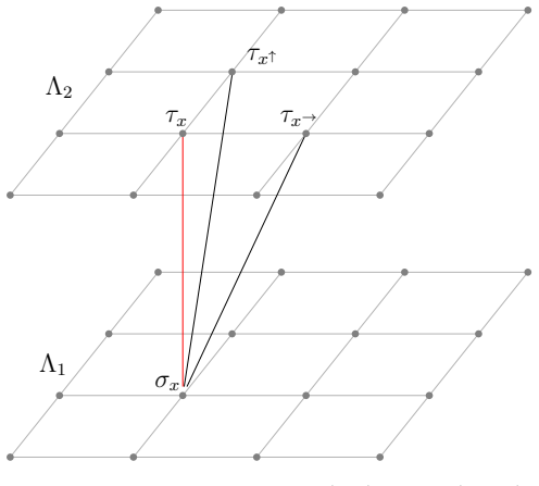
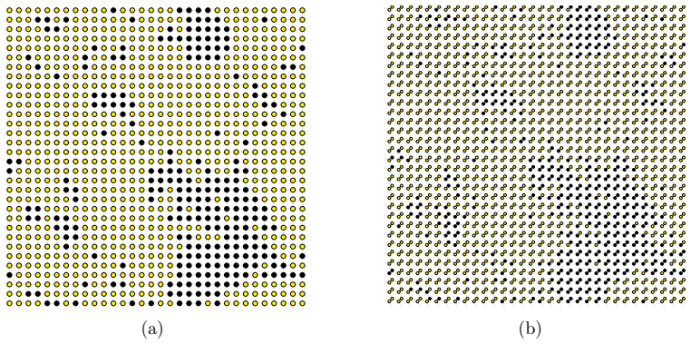
The central object is the shaken dynamics, a probabilistic cellular automaton defined as the marginal on one sublattice of an alternate parallel heat-bath dynamics on a bipartite graph. Each half-step updates all spins simultaneously with probabilities derived from a two-parameter Hamiltonian $H(\sigma,\tau) = -\sum_x [J\sigma_x(\tau_{x^\uparrow}+\tau_{x^\to})+q\sigma_x\tau_x]$, where $q$ is a self-interaction that tunes the effective lattice geometry. The load-bearing identity is the critical-curve equation $1 = 2\tanh J\tanh q + \tanh^2 J$, whose solution is $J_c(q)$; it comes from the even-subgraph expansion for the honeycomb-lattice Ising partition function. The paper uses this identity to predict where the magnetization variance should peak, and uses the partial-order-preserving update to estimate mixing via coalescence of two extremal chains.

What would settle it

Directly estimate the total-variation distance $\|\pi_s - \pi_G\|_{TV}$ from Propp-Wilson samples for $q=2.5$ on increasing lattice sizes; if the distance does not tend to zero as $|\Lambda|\to\infty$, or if the magnetization variance peaks away from $J_c(q)$ on lattices larger than $200\times200$, the central claims would be refuted.

Watch

Extended reading notes

Core claim

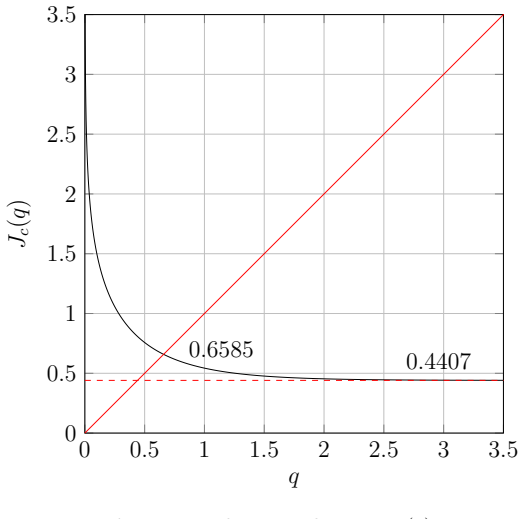
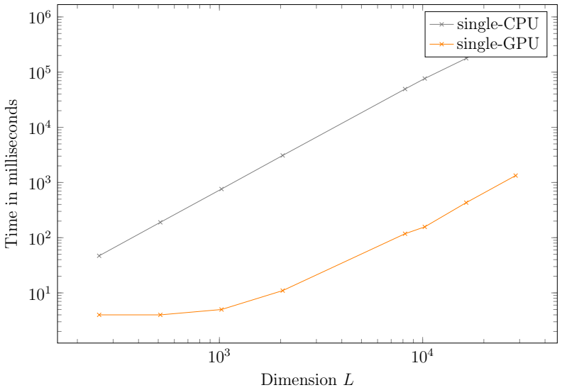
The paper claims that the shaken dynamics—a factorized, fully parallel update rule on a bipartite lattice—undergoes an order-disorder phase transition along the explicit curve $J_c(q) = \tanh^{-1}(\sqrt{\tanh^2 q + 1} - \tanh q)$, which limits to the square-lattice critical value $\tanh^{-1}(\sqrt{2}-1)\approx 0.4407$ as $q\to\infty$ and passes through the honeycomb critical point $J=q\approx 0.6585$. Using the variance of the magnetization as a phase indicator on a $200\times200$ torus, the authors locate the transition points over a grid in $(q,J)$ and find they fall on the theoretical curve. They also measure coalescence times to estimate mixing, and compare the shaken dynamics' equilibrium samples against the square-lattice Gibbs measure for magnetization and energy, concluding that for $q\ge 2.5$ the approximation is good. Two parallel implementations (multicore CPU and GPU) are benchmarked, with the GPU version running roughly 500 times faster than a single CPU core for large lattices.

Load-bearing premise

The paper assumes the companion-paper theorems are correct—the critical-curve equation and the large-$q$ convergence of the shaken equilibrium measure to the square-lattice Gibbs measure—and assumes that 300,000 warm-up steps bring the chain to equilibrium.

Editorial extensions

If this is right

The shaken dynamics serves as one parallel MCMC algorithm that can simulate the whole family of Ising models across lattice geometries by tuning only $q$ and $J$.
The critical curve is confirmed numerically, so the phase diagram of the two-parameter Hamiltonian is established by both theory and simulation.
For $q\ge2.5$, shaken-dynamics samples approximate square-lattice Gibbs samples well enough to estimate magnetization and energy at the accuracies shown.
Coalescence-time comparisons indicate the parallel alternate dynamics mixes faster per attempted spin flip than the single-spin-flip heat bath, even after volume renormalization.
The GPU implementation is roughly 500 times faster than a single CPU core for large lattices, making large-scale Monte Carlo runs practical.

Reading between the lines

Editorial extensions of the paper, not claims the author makes directly.

If the $q\ge2.5$ approximation holds in total variation and not just for the observables tested, the shaken dynamics could be a drop-in parallel replacement for single-spin-flip samplers wherever the exact Gibbs measure is not essential.
The pattern of coalescence times suggests tuning $q$ could trade bias against mixing speed; testing intermediate $q$ values (e.g., $q\in[1.5,2.5]$) by direct total-variation estimates would map that trade-off.
The even-subgraph critical-curve method might extend to other doubly periodic planar lattices, potentially producing a family of tunable parallel samplers for anisotropic Ising-type models.
A natural follow-up is to measure autocorrelation times rather than coalescence times, since the latter may be pessimistic for the variance of estimators in practice.

Share X Bluesky LinkedIn Reddit HN

Signed reviews

No signed human review yet.

Editorial analysis

A structured set of objections, weighed in public.

Desk editor's note, referee report, and a circularity audit.

Desk Editor's Note

read the letter

Colleague,

What you should know first: this is a numerical support paper for the shaken dynamics PCA introduced in the companion papers [1,2]. The genuinely new content is the numerical verification of the critical curve, the mixing-time comparisons, the correlation table, and the GPU benchmark. None of that is revolutionary, but it is useful and mostly done carefully.

The strong parts are the Propp-Wilson exact-sampling comparisons in Figs. 10-13. Those are not subject to a warm-up assumption, and they give real evidence that for q >= 2.5 the shaken dynamics equilibrium is close to the square-lattice Gibbs measure. The coalescence-time comparison with heat bath, renormalized by volume, is a fair and informative way to show that the parallel dynamics is not cheating. The correlation table qualitatively supports the anisotropy theorem from [1]. Credit where due: the numerical experiments are independent checks of the companion theorems, not fits to them.

Now the soft spots, in proportion. The stress-test note is right. Section 3.1 locates the phase transition by looking at the magnetization variance on a single 200x200 torus after a fixed 300k warm-up, with no mixing diagnostic. The paper's own Fig. 8 shows coalescence times on L=32 reaching 10^5-10^6 steps near criticality; L=200 should be slower. The text admits the warm-up 'turned out to be good enough' without any quantitative check, such as agreement from all-plus vs all-minus starts or a variance-peak stability scan. So the variance ridge in Figs. 6-7 may not be an equilibrium signal, and the numerical support for eq. (11) is weaker than the figures suggest. This concern does not affect the exact-sampling sections, so the central q>=2.5 claim survives.

Minor but real: no error bars on coalescence times, correlations, or the benchmark. The GPU speedup factor of 500 comes from one measurement, no runs shown for variance. Code is not provided, despite the promise of a Julia library. The writing has some rough edges (e.g., duplicated paragraph in the intro, 'stime stesps' typo). None of that changes the scientific content.

Bottom line: this paper deserves a serious referee, not a desk reject. The numerical work is worth publishing after the authors add mixing diagnostics for the critical-curve runs, report error bars, and ideally release code. If they address the equilibration issue, the paper is a solid contribution to computational statistical mechanics.

For the reading group I'd say maybe; it is not urgent but it is relevant if anyone cares about parallel samplers for Ising-type models. I would not cite it in my own next work, but I would point to [1,2] instead for the dynamics and to this paper as a reference for implementation details.

Referee Report

5 major / 6 minor

Summary. The manuscript presents numerical simulations of the 'shaken dynamics', a parallel probabilistic cellular automaton for the 2D Ising model on a bipartite lattice with parameters J and q. The authors estimate the critical curve Jc(q) in the (q,J) plane via magnetization-variance measurements, study coalescence times and mixing behavior, compute spin-spin correlations, compare the shaken dynamics' equilibrium measure with the Gibbs measure of the square-lattice Ising model for large q, and report CPU/GPU implementations with a benchmark. The paper is positioned as numerical support for the companion theoretical papers [1] and [2], whose predictions it aims to verify.

Significance. If the numerical evidence is quantitatively sound, the paper would provide useful independent validation of the analytical critical curve and of the claim that the shaken dynamics approximates the square-lattice Ising Gibbs measure for q≥2.5. Its strengths include the use of Propp-Wilson exact sampling for the equilibrium comparisons in Figs. 10-13, which avoids warm-up bias in those comparisons, and the concrete algorithmic description with a GPU benchmark. The central limitation is that the critical-curve identification rests on an unchecked equilibration assumption for a single lattice size, and several key quantities are reported without error bars or quantitative comparisons to the analytic predictions.

major comments (5)

[§3.1, Eq. (11)/(12), Fig. 7] The only numerical evidence for the critical curve is the variance ridge of the magnetization on a single 200×200 torus after a fixed 300,000-step warm-up from the all-minus state. This does not establish equilibration: the paper's own coalescence measurements in Fig. 9 for L=32 reach 10^5-10^6 steps near criticality, and mixing on L=200 should be slower. Provide a mixing diagnostic (e.g., agreement between all-plus and all-minus starts, or a plot of the variance peak versus warm-up length) and a quantitative measure of the distance between the observed ridge and Jc(q). Without these, the validation of Eq. (12) is weaker than Fig. 7 suggests.
[§3.1, Fig. 7] The threshold variance ≥0.03 used to center the bars in Fig. 7 is arbitrary, and no justification is given for why this threshold identifies the transition rather than merely a fixed fluctuation level. Since the height and width of the variance peak depend on lattice size, run length, and correlation time, the threshold should be justified or replaced by a more robust estimator (for example, a Binder-cumulant or finite-size-scaling analysis).
[§3.2, Figs. 8-9 and 14] Coalescence times are central to the mixing-time comparisons, yet they are reported as sample averages with no standard errors, no number of independent repetitions, and no indication of how many chains were coupled. This makes it impossible to judge whether the apparent speedups of the shaken or alternate dynamics over single-spin-flip dynamics are statistically meaningful, especially near criticality where coalescence times fluctuate strongly.
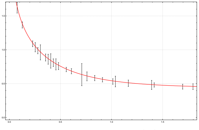
[§3.2, Figs. 10-13] The statement that 'for q≥2.5 the approximation provided by the shaken dynamics is quite good' is not backed by a quantitative distance between the shaken-dynamics observables and the Gibbs-reference values. Several panels, e.g. the energy standard deviation panels in Fig. 13, show discrepancies that appear larger than the between-algorithm scatter, and no error bars are given. Report a quantitative measure (e.g., the maximum observable bias or an estimated total-variation distance) over the plotted J values.
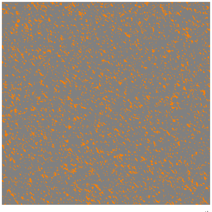
[§3.3, Table 1] The spin-spin correlation table is presented without error bars or a statement of the number of independent samples used, so the directional asymmetry conclusion and the claim that correlations decay rapidly below Jc rest on uncharacterized single-run estimates. For example, the q=0.05 supercritical row shows the SW-NE correlation at l=16 (0.739) exceeding the NW-SE value at the same distance (0.726), which is not discussed and may indicate large statistical uncertainty.

minor comments (6)

[Section 1] The paragraph beginning 'In this framework, a new PCA parameterized by J and q...' is duplicated verbatim within the Introduction.
[Section 2, after Eq. (6)] The sentence 'The critical value of βc separates the ordered phase where all the spin have the same probability... from the ordered phase where the measure is polarized' should read 'disordered phase' in the first instance.
[Section 3.1] The text says the simulations are run 'for (J,q)∈{(0,2)×(0,2)} on a 80×80 grid', while Section 4 says 80 couples of (q,J) values were simulated; please clarify whether the parameter grid has 80 points or 6400 points.
[Section 3.2, Fig. 8] Figure 8 lacks a color scale label; the reader has to infer that the color encodes the logarithm of the average coalescence time, and no units or error information are provided.
[Section 4.0.1] The phrase 'we can not go beyond105 for this GPU' appears to have a missing exponent or line break; it should read something like '10^5'.
[Section 4.0.2, Fig. 20] The benchmark plot shows single timings with no error bars or repeated measurements; since the text claims a speed-up factor of approximately 500, a statement of measurement variability would strengthen the claim.

Circularity Check

0 steps flagged · score 1.0 of 10

No circular derivation: the numerical experiments independently test the companion-paper theorems [1,2] rather than fitting or renaming them.

full rationale

The paper's central theoretical inputs are the critical curve (eq. 12), the equilibrium measure of the shaken dynamics, and the large-q approach to the square-lattice Gibbs measure. All of these are cited to the companion papers [1] and [2], which are self-citations from the same research group, and the paper explicitly describes itself as numerical support for those papers. That dependence is real: eq. (11) and eq. (12) are not re-derived here. However, the numerical program is an independent, externally falsifiable test of those theorems rather than a construction that re-imports them. Section 3.1 estimates the phase-transition location from the variance of the magnetization computed by direct simulation and compares the resulting ridge to the analytic curve; no parameter is fitted to make the ridge match eq. (12). The mixing-time and coalescence measurements are independent observables, and the Gibbs-comparison section uses Propp-Wilson exact sampling with two reference dynamics, including the standard single-spin-flip heat bath, so the shaken dynamics is compared against an external Gibbs benchmark. The warm-up time of 300,000 steps is asserted rather than quantitatively justified, and the 200x200 runs lack mixing diagnostics near criticality, but that is a correctness or statistical-risk concern, not a circularity. No equation in the paper reduces to the quantity it is claimed to predict, and no fitted constant is relabeled as a prediction. The self-citations are load-bearing for the theoretical framework, yet the numerical content gives them independent support, so the circularity burden is low. The overall score reflects the heavy reliance on companion-paper theorems while acknowledging the absence of any by-construction equivalence between inputs and outputs.

Assumptions & free parameters 0 free parameters · 4 assumptions · 0 invented entities

The paper introduces no new entities or fitted parameters. It relies on the theoretical results of the companion papers [1,2] for the critical curve and equilibrium measure, and on standard Markov chain coupling and PCA theory.

assumptions (4)

domain assumption The critical curve for the Hamiltonian (5) is given by eq. (12), from Theorem in [1].
The paper uses this analytic curve as the target for numerical verification; it is not re-derived here, only cited from [1].
domain assumption The equilibrium measure of the shaken dynamics is pi_s(sigma) = Z_sigma / Z, proved in [2].
This is the theoretical basis for comparing the shaken dynamics equilibrium with Gibbs measures; the paper cites [2].
domain assumption For large q, pi_s approaches the Gibbs measure of the square-lattice Ising model, i.e., Theorem 2.3 in [2].
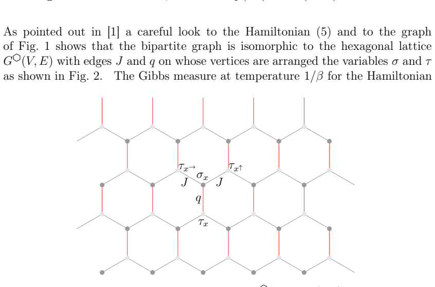
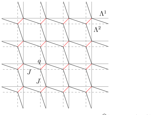
The paper's claim that q>=2.5 gives a good approximation relies on this theorem.
domain assumption The bipartite graph with q and J edges is isomorphic to the hexagonal lattice.
This justifies interpreting the dynamics as simulating honeycomb-lattice Ising models; argued in Section 2 and [1].

how reviews work

0 comments

Cite this review

Pith. "Pith review of Parallel simulation of two--dimensional Ising models using Probabilistic Cellular Automata." pith.science (2026). https://pith.science/paper/R3VGSXXF

@misc{pith2026190807341,
  author       = {Pith},
  title        = {Pith review of: Parallel simulation of two--dimensional Ising models using Probabilistic Cellular Automata},
  year         = {2026},
  howpublished = {\url{https://pith.science/paper/R3VGSXXF}},
  note         = {Machine review of arXiv:1908.07341}
}

abstract

We perform a numerical investigation of the \emph{shaken dynamics}, a parallel Markovian dynamics for spin systems with local interaction and whose transition probabilities depend on two parameters, $q$ and $J$, that tune the geometry of the underlying lattice. We determine a phase transition curve, in the $(q, J)$ plane, separating the disordered phase from the ordered one, study the mixing time of the Markov chain and evaluate the spin-spin correlations as $q$ and $J$ vary. Further, we investigate the relation between the equilibrium measure of the shaken dynamics and the Gibbs measure for the Ising model. Two different approaches are considered for the implementation of the dynamics: a multicore CPU approach, with code written in Julia and a GPU approach with code written in CUDA.

Figures

Figures reproduced from arXiv: 1908.07341 by the authors.

**Figure 1.** The lattices Λ1, Λ2 with the q (red) and J (black) interactions. As pointed out in [1] a careful look to the Hamiltonian (5) and to the graph of [PITH_FULL_IMAGE:figures/full_fig_p005_1.png] view at source ↗

**Figure 2.** The hexagonal graph G9(Λ1 ∪ Λ2, {J, q}) (5) is π2(σ, τ ) = e −βH(σ,τ) P (σ,τ)∈X ×X e −βH(σ,τ) (6) 5 [PITH_FULL_IMAGE:figures/full_fig_p005_2.png] view at source ↗

**Figure 3.** A representation of the hexagonal graph G9(Λ1 ∪ Λ2, {J, q}) that highlights the relation with the two square lattices Λ1 and Λ2 where X × X = {−1, 1} |Λ| × {−1, 1} |Λ| is the configuration space of the variable (σ, τ ). The critical value of βc separates the ordered phase where all the spin have the same probability to take the values +1 or −1 from the ordered phase where the measure is polarized [5]. Rescaling the … view at source ↗

Figures from the paper (17 more)

**Figure 4.** Figure 4: The critical curve Jc(q) the critical curve Jc(q) for the Hamiltonian (5) is the unique solution for J, q > 0 of the equation X γ∈E0(G) Y e∈γ tanh Je = X γ∈E1(G) Y e∈γ tanh Je (10) where E0(G) is the set of even subgraphs of G9 winding an even number of times around ea…

**Figure 5.** Figure 5: Average (a) and variance (b) of the magnetization as a function of J for q = 0.6585 ���� (a) ���� (b) [PITH_FULL_IMAGE:figures/full_fig_p010_5.png]

**Figure 6.** Figure 6: Average (a) and variance (b) of the magnetization on the whole (q, J) grid [PITH_FULL_IMAGE:figures/full_fig_p010_6.png]

**Figure 7.** Figure 7: The bars are centered at those points in the (q, J) plane for which the variance of the magnetization is sufficiently large (≥ 0.03). The length of the bars is proportional to the variance of the magnetization. nient to look at its mixing time. For a Markov chain (Xn)n…

**Figure 8.** Figure 8: Logarithm of the average coalescence time for values of J and q close to the critical curve where σ x is the configuration obtained from σ by flipping the spin at site u and hu(σ) = P y∼x Jσy. Also the heat bath dynamics preserves the partial ordering between configura…

**Figure 9.** Figure 9: Sample average of the coalescence time for J = q (hexagonal lattice) then, for J sufficiently large, lim |Λ|→∞ kπs − πGkTV = 0, where πG is the Gibbs measure for the Ising model on the square lattice. Therefore it makes sense to evaluate numerically the goodness of thi…

**Figure 10.** Figure 10: Sample average of the magnetization for several values of J On the other hand, we also estimated the time required to approach the equilibrium distribution by comparing the coalesce time of the shaken dynamics with those of the two other reference dynamics. Also in th…

**Figure 11.** Figure 11: Sample standard deviation of the magnetization for several values of J a spin configuration living on Λ1. In words, the theorem states that the SW-NE correlations are weaker than the NW-SE ones if the self interaction is weak. On the other hand, we expect that the SW-…

**Figure 12.** Figure 12: Sample average of the energy H(σ) for several values of J simulation on 80 couples of values (q, J) in the range of (q, J) ∈ (0, 2) × (0, 2). The Hamiltonian is defined on a square 200 × 200 lattice. Statistics are collected over 300,000 iterations. Fig.6 shows that t…

**Figure 13.** Figure 13: Sample standard deviation of the energy H(σ) for several values of J Algorithm 2 collectDL Input xσ, J, q Output f 1: f ← J(σx↓ + σx←) + qσx 2: Return f We implemented the algorithm 3 in two parallel ways. A CUDA 2 implementation of a parallel heat bath for large dim…

**Figure 14.** Figure 14: Sample average of the coalescence time (number of steps) for several values of J (a) (b) [PITH_FULL_IMAGE:figures/full_fig_p020_14.png]

**Figure 15.** Figure 15: J = 0.44, q = 3.0 The collect function computes the transition probabilities in the given direction. Each thread handles one spin on the lattice field. The principal use of the global memory is the four square spin lattice, the two configuration sigma (σ) and tau (τ )…

**Figure 16.** Figure 16: J = 0.6585, q = 0.6585 (a) (b) [PITH_FULL_IMAGE:figures/full_fig_p021_16.png]

**Figure 17.** Figure 17: J = 2.0, q = 0.03 We did not use shared memory for the random-unit. The code was written to run on the Nvidia-GPU Tesla P100 using by 16GB video memory, using 4 matrices of dimension L×L, two for the lattice spin field (single byte), and two for the collected fields a…

**Figure 18.** Figure 18: GPU sample: L = 512, J = 0.99, q = 0.5, iteration= 60th which is L 2 . For this benchmark (Fig. (20)), we used an Nvidia graphic card Tesla P-100 vs single core of the CPU Intel(R) Xeon(R) CPU E5-2698 v4 @ 2.20GHz. We measure the time for one update execution. As we h…

**Figure 19.** Figure 19: CPU sample: L = 512, J = 0.99, q = 0.5, iteration= 60th 5 Conclusions 5.1 Summary The present work is a numerical experiment on the 2D Ising model. In particular the tasks are mainly focused on the shaken dynamics, in which we used to approximate numerically the crit…

**Figure 20.** Figure 20: Running-time in function of the size L. we compare the coalescence time between the alternate and shaken dynamics on the critical line (red line in [PITH_FULL_IMAGE:figures/full_fig_p025_20.png]

Discussion (0). Continue with ORCID to comment.

Reference graph

Works this paper leans on

17 extracted references · 11 canonical work pages

[1]

Criticality of measures on 2-d Ising configurations: from square to hexagonal graphs

ValentinaApollonioetal.“Criticalityofmeasureson2-dIsingconﬁgurations: from square to hexagonal graphs”. In: (2019). eprint:arXiv:1906.02546

work page Pith review arXiv 2019
[2]

Shaken dynamics: an easy way to parallel Markov Chain Monte Carlo

Valentina Apollonio et al. “Shaken dynamics for the 2d Ising model”. In: (2019). doi: https://arxiv.org/abs/1904.06257

work page Pith review arXiv 2019
[3]

The critical temperature for the Ising model on planar doubly periodic graphs

David Cimasoni and Hugo Duminil-Copin. “The critical temperature for the Ising model on planar doubly periodic graphs”. eng. In:Electronic Journal in Probability 18.44 (2013). ID: unige:30547, pp. 1–18.url: https://archive- ouverte.unige.ch/unige:30547

work page 2013
[4]

Sampling from a Gibbs Measure with Pair Interaction by Means of PCA

Paolo Dai Pra, Benedetto Scoppola, and Elisabetta Scoppola. “Sampling from a Gibbs Measure with Pair Interaction by Means of PCA”. In:Journal of Statistical Physics 149.4 (2012), pp. 722–737.issn: 1572-9613. doi: 10. 1007/s10955-012-0612-9 . url: http://dx.doi.org/10.1007/s10955- 012-0612-9

doi:10.1007/s10955- 2012
[5]

Instabilities and Phase Transitions in the Ising Model. A Review

G. Gallavotti. “Instabilities and Phase Transitions in the Ising Model. A Review”. In:RIVISTA DEL NUOVO CIMENTO 2 (1972), pp. 133–169

work page 1972
[6]

Time-Dependent Statistics of the Ising Model

Roy J. Glauber. “Time-Dependent Statistics of the Ising Model”. In:j-J- MATH-PHYS 4.2 (Feb. 1963), pp. 294–307.issn: 0022-2488 (print), 1089- 7658 (electronic), 1527-2427.doi: https://doi.org/10.1063/1.1703954 . url: http://jmp.aip.org/resource/1/jmapaq/v4/i2/p294_s1

doi:10.1063/1.1703954 1963
[7]

From PCA’s to equilibrium systems and back

Sheldon Goldstein et al. “From PCA’s to equilibrium systems and back”. In: Communications in Mathematical Physics 125.1 (Mar. 1989), pp. 71–79. issn: 1432-0916. doi: 10.1007/BF01217769. url: https://doi.org/10. 1007/BF01217769

work page doi:10.1007/bf01217769 1989
[8]

Häggström and O.H.G

O. Häggström and O.H.G. M.Finite Markov Chains and Algorithmic Appli- cations. London Mathematical Society Student Texts. Cambridge University Press, 2002.isbn: 9780521890014.url: https://books.google.it/books? id=hpLxIJ9LwRgC. 26

work page 2002

Show all 17 references

[9]

Julia: A Fresh Approach to Numerical Computing

Stefan Karpinski et al. “Julia: A Fresh Approach to Numerical Computing”. In: SIAM Review 59 (2017), pp. 65–98.doi: http://dx.doi.org/10.1137/ 141000671

2017
[10]

Equilibrium and Non-equilibrium Ising Mod- els by Means of PCA

C. Lancia and B. Scoppola. “Equilibrium and Non-equilibrium Ising Mod- els by Means of PCA”. In:Journal of Statistical Physics 153 (Nov. 2013), pp. 641–653.doi: 10 . 1007 / s10955 - 013 - 0847 - 0. arXiv: 1307 . 2148 [math-ph]

2013
[11]

Markov Chains and Mixing Times: Second Edition

D.A.LevinandY.Peres. Markov Chains and Mixing Times: Second Edition . American Mathematical Society, 2017.isbn: 9781470429621

2017
[12]

Lindvall

T. Lindvall. Lectures on the Coupling Method . Dover Books on Mathemat- ics. Dover Publications, 2012.isbn: 9780486153247. url: https://books. google.it/books?id=gWK8AQAAQBAJ

2012
[13]

Exact Sampling with Cou- pled Markov Chains and Applications to Statistical Mechanics

James Gary Propp and David Bruce Wilson. “Exact Sampling with Cou- pled Markov Chains and Applications to Statistical Mechanics”. In:Random Struct. Algorithms 9.1-2 (Aug. 1996), pp. 223–252.issn: 1042-9832. doi: 10.1002/(SICI)1098-2418(199608/09)9:1/2<223::AID-RSA14>3.0.CO; 2-...

1996 doi
[14]

D. Ruelle. Statistical Mechanics: Rigorous Results . World Scientiﬁc, 1999. isbn:9789810238629. url: https://books.google.it/books?id=mNtWfcj% 5C_xhwC

1999
[15]

Nonuniversal critical dynamics in Monte Carlo simulations

Robert H. Swendsen and Jian-Sheng Wang. “Nonuniversal critical dynamics in Monte Carlo simulations”. In:Phys. Rev. Lett. 58 (2 Jan. 1987), pp. 86–88. doi: 10.1103/PhysRevLett.58.86. url: https://link.aps.org/doi/10. 1103/PhysRevLett.58.86

1987 doi
[16]

Collective Monte Carlo Updating for Spin Systems

Ulli Wolﬀ. “Collective Monte Carlo Updating for Spin Systems”. In:Phys. Rev. Lett. 62 (4 Jan. 1989), pp. 361–364.doi: 10.1103/PhysRevLett.62

1989 doi
[361]

url: https://link.aps.org/doi/10.1103/PhysRevLett.62.361. 27

doi

Pith tools

Reviewed August 14, 2026 · model on record in the stance chip above.

[1] [1]

Criticality of measures on 2-d Ising configurations: from square to hexagonal graphs

ValentinaApollonioetal.“Criticalityofmeasureson2-dIsingconﬁgurations: from square to hexagonal graphs”. In: (2019). eprint:arXiv:1906.02546

work page Pith review arXiv 2019

[2] [2]

Shaken dynamics: an easy way to parallel Markov Chain Monte Carlo

Valentina Apollonio et al. “Shaken dynamics for the 2d Ising model”. In: (2019). doi: https://arxiv.org/abs/1904.06257

work page Pith review arXiv 2019

[3] [3]

The critical temperature for the Ising model on planar doubly periodic graphs

David Cimasoni and Hugo Duminil-Copin. “The critical temperature for the Ising model on planar doubly periodic graphs”. eng. In:Electronic Journal in Probability 18.44 (2013). ID: unige:30547, pp. 1–18.url: https://archive- ouverte.unige.ch/unige:30547

work page 2013

[4] [4]

Sampling from a Gibbs Measure with Pair Interaction by Means of PCA

Paolo Dai Pra, Benedetto Scoppola, and Elisabetta Scoppola. “Sampling from a Gibbs Measure with Pair Interaction by Means of PCA”. In:Journal of Statistical Physics 149.4 (2012), pp. 722–737.issn: 1572-9613. doi: 10. 1007/s10955-012-0612-9 . url: http://dx.doi.org/10.1007/s10955- 012-0612-9

doi:10.1007/s10955- 2012

[5] [5]

Instabilities and Phase Transitions in the Ising Model. A Review

G. Gallavotti. “Instabilities and Phase Transitions in the Ising Model. A Review”. In:RIVISTA DEL NUOVO CIMENTO 2 (1972), pp. 133–169

work page 1972

[6] [6]

Time-Dependent Statistics of the Ising Model

Roy J. Glauber. “Time-Dependent Statistics of the Ising Model”. In:j-J- MATH-PHYS 4.2 (Feb. 1963), pp. 294–307.issn: 0022-2488 (print), 1089- 7658 (electronic), 1527-2427.doi: https://doi.org/10.1063/1.1703954 . url: http://jmp.aip.org/resource/1/jmapaq/v4/i2/p294_s1

doi:10.1063/1.1703954 1963

[7] [7]

From PCA’s to equilibrium systems and back

Sheldon Goldstein et al. “From PCA’s to equilibrium systems and back”. In: Communications in Mathematical Physics 125.1 (Mar. 1989), pp. 71–79. issn: 1432-0916. doi: 10.1007/BF01217769. url: https://doi.org/10. 1007/BF01217769

work page doi:10.1007/bf01217769 1989

[8] [8]

Häggström and O.H.G

O. Häggström and O.H.G. M.Finite Markov Chains and Algorithmic Appli- cations. London Mathematical Society Student Texts. Cambridge University Press, 2002.isbn: 9780521890014.url: https://books.google.it/books? id=hpLxIJ9LwRgC. 26

work page 2002