REVIEW 4 major objections 6 minor 28 references
From Pixels to CSI: Distilling Latent Dynamics For Efficient Wireless Resource Management
T0 review · 4 major / 6 minor · reviewed 2026-08-06 · deepseek-v4-flash
Pith's one-line read A remote controller that learns latent dynamics of both the visual task and the wireless channel schedules transmissions at favorable moments, cutting transmit power by about half without losing control performance.
desk verdict Coupled control/wireless JEPA proof of concept with a sensible cross-modal distillation idea, but the power-saving headline rests on a deterministic synthetic channel and needs stronger evidence. read the letter →
The pith
A machine-rendered reading of the paper's core claim, the machinery that carries it, and where it could break.
The reading
What carries the argument
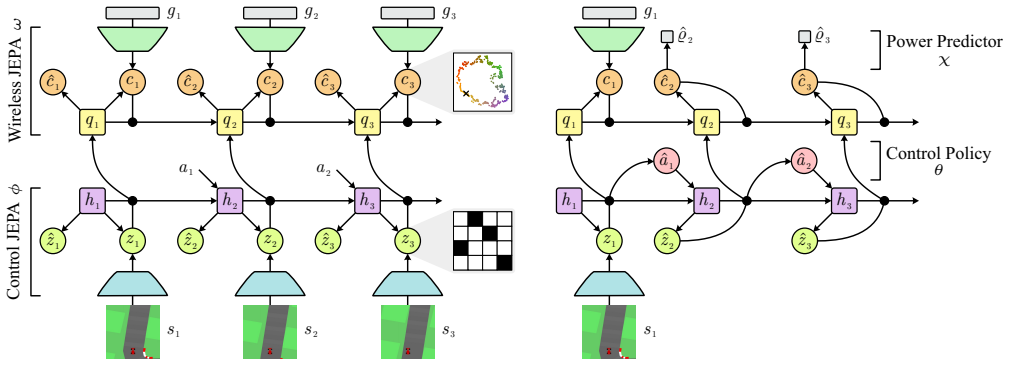
The load-bearing mechanism is a pair of coupled Joint Embedding Predictive Architectures (JEPAs), where one model's latent state conditions the other. The control JEPA, built from an image encoder, a recurrent state-space model (RSSM) with a deterministic GRU state and a discrete stochastic latent variable, plus reward and termination predictors, learns control dynamics from pixels without reconstructing the images. The wireless JEPA, built from a channel encoder and a recurrent prediction network, embeds CSI into low-dimensional vectors and predicts future embeddings, with its hidden state conditioned on the control JEPA's latent state; a stop-gradient EMA target prevents representation collapse. This cross-modal conditioning is what lets the controller convert an imagined image trajectory into an imagined channel trajectory, and it is what the power predictor uses to choose cheap transmit slots.
What would settle it
Render the same car racing scene with a randomized fading component added on top of the position-based channel and rerun the evaluation; if the gap to the power-agnostic baseline drops from the reported 3 dB toward zero, or the normalized return falls below the no-prediction baseline, the central claim that latent control states suffice to predict favorable CSI is refuted.
Extended reading notes
Core claim
On the paper's own terms, the central discovery is that future channel state information can be predicted from predicted control states, and that this cross-modal link can be learned in latent space without reconstructing pixels. The authors show that the latent representation produced by a control JEPA, trained with a discrete recurrent state-space model, carries enough information about the device's motion to drive a wireless JEPA's forecasts of CSI embeddings several steps ahead. The controller uses those forecasts to schedule the next transmission at the slot with the lowest estimated required power and to compute the power level that meets the SNR constraint, while an actor-critic policy on the latent states keeps the control task running during unscheduled slots. Results show that this architecture achieves a normalized return close to that of no-prediction baselines up to roughly 10 prediction steps, while using about 50 percent less transmit power than a power-agnostic scheduler at short horizons and 40 percent less at longer horizons.
Load-bearing premise
The load-bearing premise is that the car's latent control state contains all information needed to predict future channel state, because in the simulation the channel is rendered deterministically from position; if real channels also depend on fast fading, interference, or other unobserved factors, the wireless JEPA forecasts and the claimed power savings would degrade.
Editorial extensions
If this is right
- The controller can operate for horizons of about 10 time steps without receiving fresh images, using imagined latent states for both action selection and scheduling, while keeping control return comparable to always-transmitting baselines.
- Transmit power can be allocated per slot by evaluating predicted CSI embeddings against the SNR constraint, so scheduling and power control emerge from the same latent model instead of separate channel estimators.
- Sending a small block of consecutive samples when communicating, here κ=4, improves the control return at long horizons with only about 0.4 dB extra average power compared with κ=3.
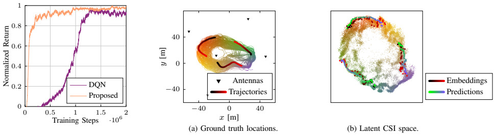
- The learned CSI embeddings preserve the spatial structure of the environment, meaning the latent wireless model generalizes along the car's trajectory rather than memorizing discrete channel states.
- Because the JEPA representations omit redundant pixel detail, policy learning converges faster than model-free DQN, reaching high normalized returns in under half a million training steps.
Reading between the lines
- The paper leaves implicit that its power savings are an upper bound for realistic deployments: the simulation renders the channel deterministically from the car's position, so if fast fading, interference, or other factors are added, the wireless JEPA would need extra conditioning inputs or a stochastic channel model to keep the same savings.
- A natural extension is to treat the coupled JEPAs as a lightweight digital twin of both the physical and radio environments, using the same latent space to drive control, scheduling, and power allocation in networked autonomy.
- A testable next step is to run the same pipeline on real channel traces or in a multi-user setting with shared resources, where the claimed 50 percent power reduction would have to be re-measured against contention and interference rather than free-space ray tracing.
- One could add a confidence estimate to the wireless predictions and trigger a fallback transmission when the imagined channel is uncertain, trading a little power to avoid the errors that would otherwise grow at long prediction horizons.
Editorial analysis
A structured set of objections, weighed in public.
Referee Report
Summary. The paper proposes a coupled JEPA framework for remote control of a device whose state is observed as images, with the goal of minimizing uplink transmit power while maintaining control performance. A control JEPA learns latent control dynamics from pixels, and a wireless JEPA learns latent CSI dynamics conditioned on the control JEPA's latent state via cross-modal conditioning. On top of these, the authors train an RL policy (actor-critic) from imagined latent trajectories and a power predictor that estimates the transmit power required for future slots, enabling the controller to schedule transmissions at low-power time slots. The method is evaluated on a synthetic pipeline combining the Car Racing gym environment with Sionna ray tracing, reporting roughly 50% transmit power savings (3 dB) at short horizons and 40% (2.2 dB) at longer horizons relative to a power-agnostic baseline, with comparable normalized control return.
Significance. If the results are robust, the paper makes a useful contribution by showing how self-supervised latent dynamics models (JEPAs) can be extended across modalities (pixels and CSI) for joint control and communication optimization. The idea of distilling control-latent information into a wireless dynamics model is interesting and goes beyond prior work that assumes access to raw velocity or known control dynamics. The paper also provides a fairly complete system architecture and reproducible hyperparameters. However, the significance is tempered by the fact that the central quantitative claim is established only in a deterministic, fully observed synthetic channel scenario, and by the absence of quantitative prediction-error metrics and statistical confidence in the reported gains. The contribution is a proof of concept rather than a demonstrated general resource-management solution.
major comments (4)
- [Section IV-A, Appendix A] The wireless channel is rendered deterministically from the car position ('the device's position is replicated from gym to render its wireless channel'), so the latent control state contains, in principle, all information needed to predict CSI. Consequently, the headline claim of 'over 50% transmit power reduction' is demonstrated only in a noiseless, fully observed channel setting; real channels with fast fading, interference, or other unobserved factors are not exercised. Please add a stochastic channel component (e.g., Rician fading or shadowing) or explicitly scope the claim to deterministic line-of-sight-like channels and discuss how the cross-modal predictor would cope with unobserved channel factors.
- [Section IV-B, Fig. 5b] The wireless JEPA's prediction quality is evaluated only qualitatively in the latent space (Fig. 5b), with no quantitative metric such as normalized MSE between predicted and true CSI embeddings, or between predicted and actual required transmit power, as a function of horizon. Since the power savings rely entirely on the accuracy of these predictions, the mechanism is not directly validated. Please report a quantitative CSI-prediction error and, if possible, the resulting scheduling accuracy.
- [Figures 4-6] All results are shown as single curves without error bars, confidence intervals, or multiple random seeds. Deep RL and self-supervised JEPA training are high-variance, and the reported 3 dB/2.2 dB savings and return differences could be within run-to-run variation. Please repeat the experiments with several seeds and report mean and variance (e.g., shaded intervals) for the key comparisons.
- [Section IV-B, baseline comparison] The transmit-power savings are measured against a 'power agnostic' baseline that schedules at the end of the prediction horizon without considering power, and against no-prediction schemes. There is no oracle or lower-bound baseline that schedules at the true lowest-power slot (knowing the channel perfectly), so the absolute quality of the learned scheduler is unknown. Adding an oracle scheduler or an offline optimal schedule would contextualize the 50% claim and indicate how much of the gain is due to the learned latent dynamics versus simply exploiting the deterministic geometry.
minor comments (6)
- [Eq. (1b), Eq. (8)] The symbol SNR is used both as the instantaneous signal-to-noise ratio (SNRt) and as a threshold in constraint (1b); the threshold is never defined. Please introduce a distinct symbol, e.g., SNR_thr, and use it consistently in Eq. (8).
- [Section IV-B, page 6] The phrase 'saving 3 times its transmit power' is ambiguous; it should read 'reducing transmit power by a factor of three' or 'using one-third of the transmit power'.
- [Section III-B, first paragraph] 'Our model is variation of the recently proposed wireless JEPA' should be 'Our model is a variation of the recently proposed wireless JEPA'.
- [Appendix A, Table I] The prediction horizon H used in experiments varies from 2 to 15, while Table I lists H = 50 as a general hyperparameter. Please clarify whether 50 is the training horizon used during JEPA training and how the evaluation horizons relate to it.
- [Fig. 5 caption] The phrase 'We use gradient coloring to identify local neighborhoods' is vague; please specify the color mapping and what exactly the predicted points represent in the latent space.
- [References and text] In the text, reference [11] is referred to as 'Time-series jepa'; consider capitalizing 'JEPA' consistently. Also, in the fourth paragraph of Section I, 'In this work, we propose a novel data-driven framework' is repeated nearly verbatim in the conclusion; consider tightening the introduction.
Circularity Check
No circularity: the power-saving claim is an experimental outcome, not a construction-level identity.
full rationale
The paper's claimed derivation chain is self-contained. The control JEPA is trained with the RSSM-style loss (2)-(3) on image observations and rewards, independent of the CSI modality. The wireless JEPA is trained with loss (4) to minimize the MSE between predicted and actual (EMA-target) CSI embeddings, conditioned on frozen control-latent features; its training target is not a function of the power predictor or of the final scheduling decision. The power predictor (8) is supervised by ground-truth values SNR·σ²/|g_t|², and the reported 50% power saving is an experimental comparison against a power-agnostic scheduler in the same simulated environment, not a quantity that is forced by construction. The self-citations [11] and [15] are prior architectural precedents (time-series JEPA and wireless JEPA) but are not used to justify the central result; the paper's contribution is the cross-modal coupling learned from data. The main limitation is external validity: in the Sionna setup the CSI is a deterministic function of position, which makes the cross-modal prediction task easier, but this is a scope concern, not a circularity. No equation reduces to its own input, and no fitted parameter is renamed as a prediction.
Assumptions & free parameters
free parameters (3)
- Prediction horizon H =
50 (training), 2-15 (evaluation)
- Scheduling parameters kappa and tau =
kappa=4, tau=2 and kappa=3, tau=1 variants
- KL scale beta and balancing mu =
beta=0.5, mu=0.8
assumptions (3)
- domain assumption The wireless channel is a deterministic function of the device's position within the Sionna scene.
- domain assumption The controller has access to an offline experience dataset with paired image states and CSI for training all networks before deployment.
- domain assumption The learned latent representations are sufficient for both policy learning and power prediction.
Cite this review
Pith. "Pith review of From Pixels to CSI: Distilling Latent Dynamics For Efficient Wireless Resource Management." pith.science (2026). https://pith.science/paper/R62JUJC7
@misc{pith2026250616216,
  author       = {Pith},
  title        = {Pith review of: From Pixels to CSI: Distilling Latent Dynamics For Efficient Wireless Resource Management},
  year         = {2026},
  howpublished = {\url{https://pith.science/paper/R62JUJC7}},
  note         = {Machine review of arXiv:2506.16216}
}
read the original abstract
In this work, we aim to optimize the radio resource management of a communication system between a remote controller and its device, whose state is represented through image frames, without compromising the performance of the control task. We propose a novel machine learning (ML) technique to jointly model and predict the dynamics of the control system as well as the wireless propagation environment in latent space. Our method leverages two coupled joint-embedding predictive architectures (JEPAs): a control JEPA models the control dynamics and guides the predictions of a wireless JEPA, which captures the dynamics of the device's channel state information (CSI) through cross-modal conditioning. We then train a deep reinforcement learning (RL) algorithm to derive a control policy from latent control dynamics and a power predictor to estimate scheduling intervals with favorable channel conditions based on latent CSI representations. As such, the controller minimizes the usage of radio resources by utilizing the coupled JEPA networks to imagine the device's trajectory in latent space. We present simulation results on synthetic multimodal data and show that our proposed approach reduces transmit power by over 50% while maintaining control performance comparable to baseline methods that do not account for wireless optimization.
Figures


Figures from the paper (2 more)

Reference graph
Works this paper leans on
-
[11]
Time-series jepa for predictive remote control under capacity-limited networks,
A. M. Girgis, A. Valcarce, and M. Bennis, “Time-series jepa for predictive remote control under capacity-limited networks,” arXiv preprint arXiv:2406.04853, 2024
arXiv 2024
-
[1]
Extreme ultra-reliable and low-latency communication,
J. Park, S. Samarakoon, H. Shiri, M. K. Abdel-Aziz, T. Nishio, A. Elgabli, and M. Bennis, “Extreme ultra-reliable and low-latency communication,” Nature Electronics, vol. 5, no. 3, pp. 133–141, 2022
work page 2022
-
[2]
Age of loop for wireless networked control system in the finite blocklength regime: Average, variance and outage probability,
J. Cao, X. Zhu, S. Sun, P. Popovski, S. Feng, and Y . Jiang, “Age of loop for wireless networked control system in the finite blocklength regime: Average, variance and outage probability,” IEEE Transactions on Wireless Communications , vol. 22, no. 8, pp. 5306–5320, 2023
2023
-
[3]
Minimizing age of information in vehicular networks,
S. Kaul, M. Gruteser, V . Rai, and J. Kenney, “Minimizing age of information in vehicular networks,” in 2011 8th Annual IEEE communications society conference on sensor , mesh and ad hoc communications and networks . IEEE, 2011, pp. 350–358
work page 2011
-
[4]
A. M. Girgis, J. Park, M. Bennis, and M. Debbah, “Predictive control and communication co-design via two-way gaussian process regression and aoi-aware scheduling,” IEEE Transactions on Communications , vol. 69, no. 10, pp. 7077–7093, 2021
work page 2021
-
[5]
Task-oriented prediction and communication co-design for haptic communications,
B. Kizilkaya, C. She, G. Zhao, and M. A. Imran, “Task-oriented prediction and communication co-design for haptic communications,” IEEE Transactions on V ehicular Technology, vol. 72, no. 7, pp. 8987–9001, 2023
work page 2023
-
[6]
Open x-embodiment: Robotic learning datasets and rt-x models : Open x-embodiment collaboration0,
A. O’Neill, A. Rehman, A. Maddukuri, A. Gupta, A. Padalkar, A. Lee, A. Pooley, A. Gupta, A. Mandlekar, A. Jain et al., “Open x-embodiment: Robotic learning datasets and rt-x models : Open x-embodiment collaboration0,” in 2024 IEEE International Conference on Robotics and Automation (ICRA) , 2024, pp. 6892–6903
work page 2024
-
[7]
A path towards autonomous machine intelligence version 0.9. 2, 2022-06-27,
Y . LeCun, “A path towards autonomous machine intelligence version 0.9. 2, 2022-06-27,” Open Review, vol. 62, no. 1, pp. 1–62, 2022
2022
Show all 28 references
-
[8]
Mastering atari with discrete world models,
D. Hafner, T. P. Lillicrap, M. Norouzi, and J. Ba, “Mastering atari with discrete world models,” in International Conference on Learning Representations , 2021
2021
-
[9]
Mastering diverse domains through world models,
D. Hafner, J. Pasukonis, J. Ba, and T. Lillicrap, “Mastering diverse domains through world models,” arXiv preprint arXiv:2301.04104 , 2023
2023 arXiv
-
[10]
Daydreamer: World models for physical robot learning,
P. Wu, A. Escontrela, D. Hafner, P. Abbeel, and K. Goldberg, “Daydreamer: World models for physical robot learning,” in Conference on robot learning . PMLR, 2023, pp. 2226–2240
2023
-
[12]
Learning latent dynamics for planning from pixels,
D. Hafner, T. Lillicrap, I. Fischer, R. Villegas, D. Ha, H. Lee, and J. Davidson, “Learning latent dynamics for planning from pixels,” in International conference on machine learning . PMLR, 2019, pp. 2555–2565
2019
-
[13]
Batch normalization: Accelerating deep network training by reducing internal covariate shift,
S. Ioffe and C. Szegedy, “Batch normalization: Accelerating deep network training by reducing internal covariate shift,” in Proceedings of the 32nd International Conference on Machine Learning , vol. 37. PMLR, 2015, pp. 448–456
2015
-
[14]
Blast: Latent dynamics models from bootstrapping,
K. Paster, L. E. McKinney, S. A. McIlraith, and J. Ba, “Blast: Latent dynamics models from bootstrapping,” in Deep RL Workshop NeurIPS , 2021
2021
-
[15]
Learning latent wireless dynamics from channel state information,
C. Bou Chaaya, A. M. Girgis, and M. Bennis, “Learning latent wireless dynamics from channel state information,” IEEE Wireless Communications Letters, vol. 14, no. 2, pp. 489–493, 2025
2025
-
[16]
Simple statistical gradient-following algorithms for connectionist reinforcement learning,
R. J. Williams, “Simple statistical gradient-following algorithms for connectionist reinforcement learning,” Machine learning, vol. 8, pp. 229–256, 1992
1992
-
[17]
Gymnasium: A standard interface for reinforcement learning environments,
M. Towers, A. Kwiatkowski, J. Terry, J. U. Balis, G. De Cola, T. Deleu, M. Goulao, A. Kallinteris, M. Krimmel, A. KG et al., “Gymnasium: A standard interface for reinforcement learning environments,” arXiv preprint arXiv:2407.17032 , 2024
2024 arXiv
-
[18]
Sionna: An open-source library for next-generation physical layer research,
J. Hoydis, S. Cammerer, F. A. Aoudia, A. Vem, N. Binder, G. Marcus, and A. Keller, “Sionna: An open-source library for next-generation physical layer research,” arXiv preprint arXiv:2203.11854 , 2022
2022 arXiv
-
[19]
Human-level control through deep reinforcement learning,
V . Mnih, K. Kavukcuoglu, D. Silver, A. A. Rusu, J. Veness, M. G. Bellemare, A. Graves, M. Riedmiller, A. K. Fidjeland, G. Ostrovskiet al., “Human-level control through deep reinforcement learning,” Nature, vol. 518, no. 7540, pp. 529–533, 2015. APPENDIX A HYPERPARAMETERS A. S...
2015
-
[20]
All layers are followed by a layer normalization and ELU activation
Image encoder: Three convolutional layers with (16, 32, 64) channels, kernels (8, 4, 2) and stride (4, 2, 2), followed by two linear layers with (1024, 256) neurons, with output size of 400. All layers are followed by a layer normalization and ELU activation
-
[21]
Its input (at−1, zt−1) are fed to a linear layer with 300 neurons followed by a layer normalization and ELU activation
RSSM recurrent network: A GRU with a hidden state ht of size 300. Its input (at−1, zt−1) are fed to a linear layer with 300 neurons followed by a layer normalization and ELU activation
-
[22]
RSSM representation network: A linear layer with 400 neurons that receives the image features and the recurrent state (xt, ht) followed by a batch normalization and ELU activation, then another linear layer with 400 neurons that outputs the 32 × 32 logits of the stochastic state zt
-
[23]
RSSM dynamics network: A linear layer with 400 neurons that receives the recurrent state ht followed by a layer normalization and ELU activation, then another linear layer with 400 neurons that outputs the 32 × 32 logits of the stochastic state zt
-
[24]
Reward/Termination prediction networks: Three layer MLPs with 100 neurons per layer, and each layer is followed by a layer normalization and ELU activation
-
[25]
Actor/Critic network: Three layer MLP with 100 neurons per layer, and each layer is followed by a layer normalization and ELU activation
-
[26]
Channel encoder network: Five layer MLP with (1024, 512, 256, 128, 64) neurons, and each layer is followed by a batch normalization and ReLU activation
-
[27]
Channel prediction network: A GRU with a recurrent state size of 256 and its output is fed to two linear layers with (64, 16) neurons
-
[28]
Power prediction network: Three layer MLP with 100 neurons per layer, and each layer is followed by a ReLU activation
Reviewed August 6, 2026 · model on record in the stance chip above.
Discussion (0). Continue with ORCID to comment.