REVIEW 3 major objections 4 minor 53 references
DynaNet: Neural Kalman Dynamical Model for Motion Estimation and Prediction
T0 review · 3 major / 4 minor · reviewed 2026-08-14 · deepseek-v4-flash
Pith's one-line read Replacing an LSTM with a differentiable Kalman filter on learned features improves motion estimation and prediction.
desk verdict Clever hybrid, but the stability proof doesn't apply to the implemented system—and the empirical claims need more support. read the letter →
The pith
A machine-rendered reading of the paper's core claim, the machinery that carries it, and where it could break.
The reading
What carries the argument
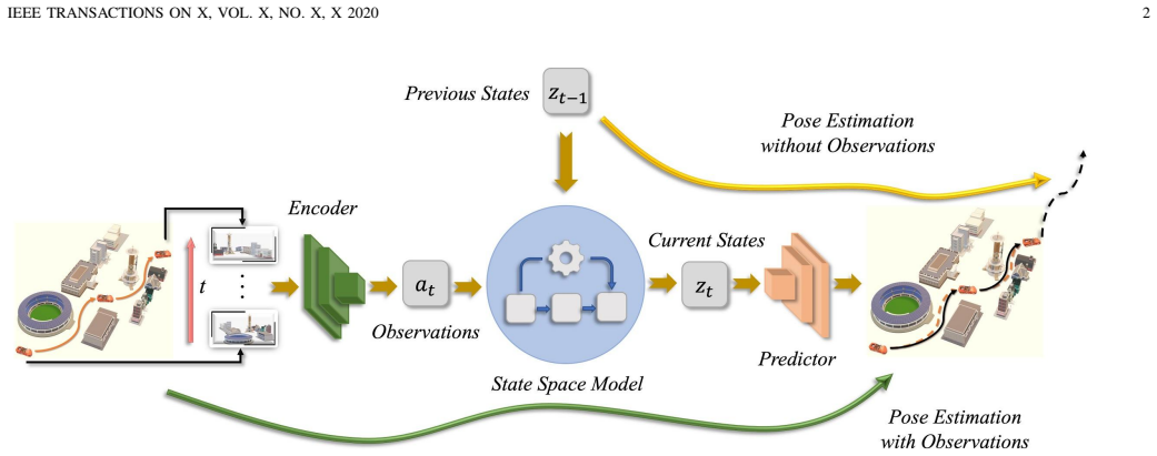
The central object is the neural Kalman dynamical model: a differentiable Kalman filter applied to latent feature states rather than hand-specified physical states. The transition matrix $A_t$ is produced by an LSTM conditioned on previous latent states in the deterministic version, or sampled from a Dirichlet distribution with LSTM-generated concentration $\alpha$ in the resampled version. An encoder emits both features $a_t$ and observation noise $R_t$, while process noise $Q_t$ is also learned, so the Kalman filter's predict and update equations propagate the mean and covariance end-to-end. The Dirichlet construction is what the stability argument relies on: because all entries of $A$ are positive and sum to one, the induced row-sum norm is less than one, so products of transition matrices contract and the state converges to zero as the horizon grows.
What would settle it
Inspect the tensor produced by the transition-generation block described in the appendix: if it is a vector of length 128 per sample rather than a $128\times128$ matrix, the implemented transition is diagonal, so a perturbation in one latent coordinate can never drive another. Then the stability proof as written does not govern the implemented model, and a direct comparison of the diagonal implementation against a full-matrix variant on the same odometry benchmark would show whether the missing off-diagonal coupling changes the reported accuracy.
Extended reading notes
Core claim
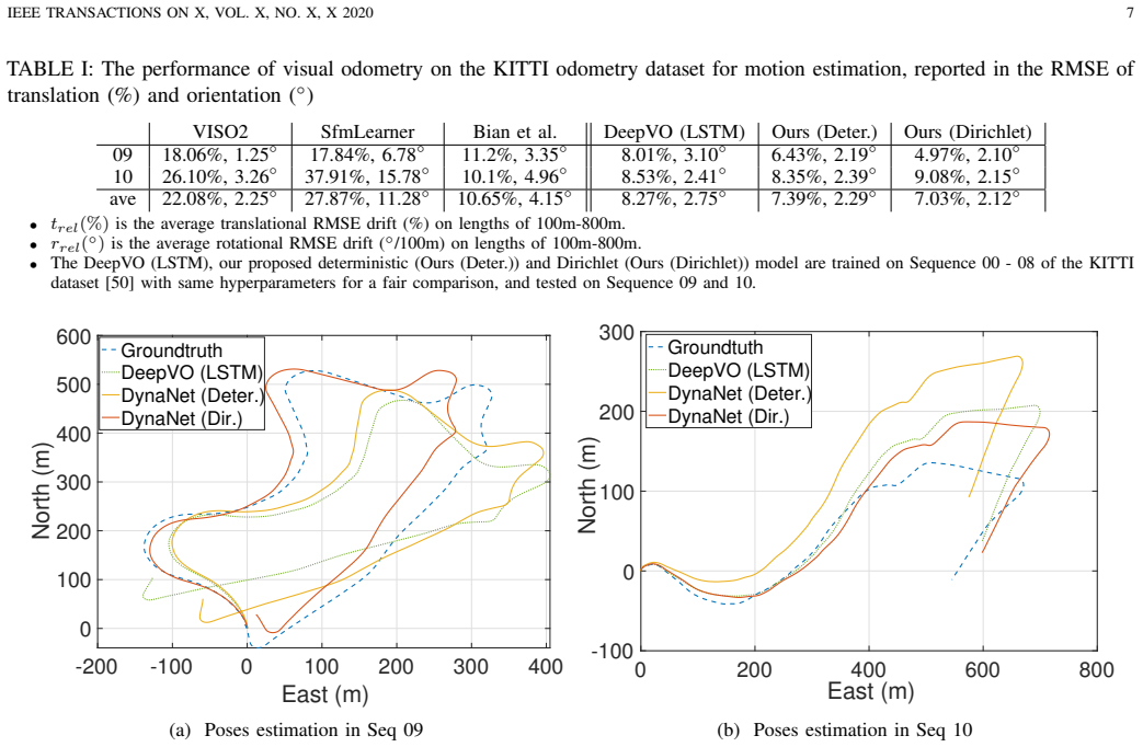
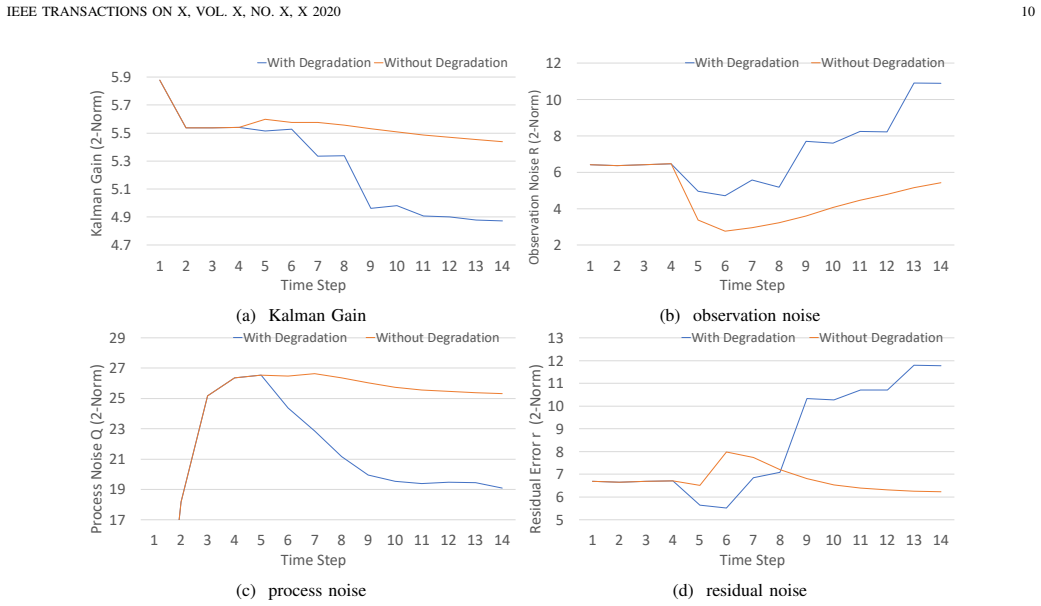
DynaNet's central claim is that a differentiable Kalman filter applied to learned latent features is a better state estimator than the LSTM it replaces. The latent state evolves as $z_t = A_t z_{t-1}$, with the time-varying transition matrix $A_t$ emitted by an LSTM; a second variant resamples $A_t$ from a Dirichlet distribution with LSTM-generated concentration so that the learned dynamics are asymptotically stable. The Kalman filter propagates a mean and covariance through predict and update steps, fusing the encoder's features and their uncertainties. On visual odometry the paper reports average translation/rotation RMSE improving from $8.27\%/2.75^\circ$ (LSTM baseline) to $7.03\%/2.12^\circ$ (Dirichlet DynaNet); on visual-inertial odometry the deterministic version improves average translation RMSE from $6.44\%$ to $5.47\%$; and in prediction without observations the Dirichlet model beats LSTM baselines. The paper also claims the Kalman gain acts as an interpretable failure signal: as input images are increasingly corrupted, the gain and process noise fall while observation noise and residual error rise, even though such corruption was not seen in training.
Load-bearing premise
The results stand or fall on the assumption that the latent features describing motion evolve linearly as $z_t = A_t z_{t-1}$, with a transition matrix generated by the recurrent network in exactly the form the stability proof requires.
Editorial extensions
If this is right
- Odometry accuracy improves without changing the encoder or pose predictor, so the gain comes specifically from replacing the LSTM state estimator with the Kalman filter module.
- The Dirichlet-resampled transition yields the largest gains in long-horizon motion prediction, consistent with the claim that enforcing stability prevents divergent extrapolation.
- The emission matrix $H$ can be set to select only the observed feature dimensions, so the same model handles missing visual or inertial cues by relying on the predicted prior state.
- The learned noise matrices $Q$, $R$, the residual error, and the Kalman gain provide a per-timestep signal about measurement quality, enabling failure indication without retraining.
- Because training minimizes a loss that compares both posterior and prior predictions to ground truth, the model is explicitly trained to predict well even when no observation arrives.
Reading between the lines
- The paper does not propose a decision threshold; a natural extension would be to calibrate the Kalman gain norm or innovation norm against labelled sensor faults and use it as a trigger for re-initialisation or handoff in autonomous systems.
- Because the implementation details list the transition output as a 128-dimensional vector rather than a $128\times128$ matrix, it is an open question whether the implemented model is diagonal; if so, the full-matrix stability proof is not the mechanism at work, and a full-matrix variant would be the cleaner test of the Dirichlet claim.
- The same Kalman-on-latent-features design should transfer to other partially observed dynamical systems, such as pedestrian trajectory forecasting or sensor networks with dropout, where the emission matrix already provides a natural missing-data mechanism.
Signed reviews
Editorial analysis
A structured set of objections, weighed in public.
Referee Report
Summary. The paper proposes DynaNet, a hybrid deep-learning and state-space model for motion estimation and prediction. The architecture combines a CNN encoder that extracts latent features from raw observations, an LSTM-based transition model that generates a time-varying transition matrix (either deterministically or by resampling from a Dirichlet distribution), and a differentiable Kalman filter that performs recursive state estimation on the feature space. The claimed contributions are end-to-end learning of a linear-like dynamical model, improved accuracy and robustness over LSTM baselines on visual odometry, visual-inertial odometry and motion prediction, and interpretability via the Kalman gain as a failure indicator. Experiments on KITTI sequences show that DynaNet outperforms DeepVO and VINet on several metrics, and the interpretability study shows that the Kalman gain decreases with image degradation.
Significance. If the claims hold, DynaNet is a useful contribution to interpretable deep state-space models for motion estimation, with practical relevance to safety-critical autonomous driving. The idea of jointly learning the Kalman filter parameters (transition, process noise, observation noise) from raw data and using the innovation/gain for online failure detection is appealing and goes beyond typical black-box RNN baselines. The paper provides a detailed appendix with exact layer specifications, which aids reproducibility. The empirical evaluation covers three tasks with public benchmarks and shows consistent gains in most settings. However, the central theoretical claims currently do not match the implemented system, as the appendix reveals a diagonal implementation while the theory and stability proof require a full matrix. This gap must be resolved before the paper can be accepted.
major comments (3)
- [Appendix A, Eq. (2), Eqs. (8)-(12)] The implementation in Appendix A (Tables V and VI) stores the transition matrix A, process noise Q, observation noise R, and covariance P all as B×128 vectors, which is only consistent with a diagonal (elementwise) transition model. In contrast, Eq. (2) and the stability proof in Eqs. (8)-(12) treat A as a full d×d matrix with strictly positive entries. The paper never states that the implemented model is diagonal, and the SDC universality argument f(z)=A(z)z in Section III does not hold for a diagonal A. Moreover, the proof's condition A(i,j)>0 for all i,j is not satisfied by a diagonal matrix, so the stability proof as written does not apply to the evaluated system. The authors must either (i) explicitly reformulate DynaNet as a diagonal state-space model, prove stability for that case (a diagonal A with positive diagonal entries summing to 1 is indeed contractive), and adjust the claims about representing general nonlinear dynamics, or (ii) implement the full-matrix model and update the appendix and experiments accordingly. This is a load-bearing discrepancy between the stated theory and the implemented system.
- [Section IV-B, Table II] In the visual-inertial odometry results, the proposed Dirichlet model has an average orientation error of 2.01°, which is worse than VINet's 1.70°, and on Sequence 10 VINet's orientation error (1.39°) is lower than both DynaNet variants. The sentence in Section IV-C that 'our proposed models outperform VINet with 2-layers LSTMs' is therefore too strong; it holds for translation on average but not for orientation. The authors should qualify the claim by specifying which metrics and sequences support it.
- [Section IV-B, Table I and Section IV-A-2] The claim that the only difference between DynaNet and DeepVO is the state estimation part is not exact, because DeepVO uses a two-layer LSTM while the DynaNet transition module uses a one-layer LSTM plus the Kalman filter. This should be clarified so that the comparison is understood as a strong baseline with a different recurrent architecture, rather than a perfectly controlled ablation.
minor comments (4)
- [Section IV-E, Figure 9] The text says 'The decreasing process noise (d) indicates...', but panel (d) in Figure 9 is the residual error, not the process noise; the process noise is panel (c). Please correct the cross-reference.
- [Throughout] There are several typos and grammar issues, e.g., 'different' for 'difference' in Section IV-B, 'vavigation' in the Table III caption, 'hyberparameters' in Section IV-B, and 'them we evaluated them' in Section IV-B. A thorough proofreading pass is needed.
- [Section IV] The experimental results are reported without any statistical significance measures, error bars, or multiple runs. Since the proposed models and baselines are stochastic (especially the Dirichlet resampling), reporting the variance across several random seeds would strengthen the empirical claims.
- [Section III-B-2] The sentence 'The latent features are extracted by the encoder, which ensures the transition states strictly positive' is ambiguous: the positivity refers to the latent states z, not the transition matrix A. Please rephrase to avoid confusion.
Circularity Check
No significant circularity: the stability guarantee is an explicit construction, the Kalman recursion is standard, and the empirical gains are evaluated on held-out sequences against external and ablation baselines.
full rationale
The paper's derivation chain is self-contained at the equation level. Equation (2) invokes a standard SDC existence result [44] from the external controls literature, and Eqs. (13)-(14) are the textbook Kalman predict/update recursions. The Dirichlet stability argument (Eqs. (8)-(12)) is an explicit design constraint rather than a fitted prediction: the paper states that it 'propose[s] to resample the transition function from a Dirichlet distribution to ensure system stability,' and the proof verifies directly that a transition matrix with positive entries summing to one has infinity norm less than one. No test-set quantity is fit and then renamed a prediction; Eq. (17) trains both posterior and prior outputs against ground truth, and the prediction experiments in Section IV-D are evaluated on held-out KITTI sequences. The comparisons include external baselines (SfmLearner, Bian et al., VISO2, VINS-Mono, OKVIS) alongside the authors' own DeepVO/VINet, so the self-citations are not load-bearing evidence for the central claim. The only substantive concern is a correctness gap in Appendix A, where A, Q, R and P are all given as B x 128 vectors, implying an elementwise/diagonal transition rather than the full d x d matrix assumed in Eqs. (2)-(12); this would invalidate the applicability of the stability proof to the implemented system, but it is an implementation-representation mismatch, not a circular reduction of a result to its inputs.
Assumptions & free parameters
free parameters (6)
- Latent state dimension d =
128
- Training sequence length =
5 frames
- Prediction horizons evaluated =
5 and 10 steps
- Tiny random positive number for state positivity =
not specified
- Gaussian noise added to Dirichlet concentration =
not specified
- Initial state covariance P_0 =
not specified
assumptions (5)
- standard math Any continuous differentiable function f with f(0)=0 admits a state-dependent coefficient form f(z) = A(z) z.
- domain assumption The latent state transition is Markovian and the measurement model is linear with additive Gaussian noise.
- domain assumption If a transition matrix is sampled from a Dirichlet distribution over its elements, the resulting linear system is BIBO/asymptotically stable.
- domain assumption The learned observation noise covariance R and process noise covariance Q are valid positive-semidefinite covariance matrices, and the Kalman update is differentiable through the inverse in S_t.
- domain assumption The encoder can extract latent states that evolve according to a linear-like rule with the LSTM-generated A, and the pose predictor can decode these latent states into 6-DoF poses.
Cite this review
Pith. "Pith review of DynaNet: Neural Kalman Dynamical Model for Motion Estimation and Prediction." pith.science (2026). https://pith.science/paper/RHNJFVAI
@misc{pith2026190803918,
  author       = {Pith},
  title        = {Pith review of: DynaNet: Neural Kalman Dynamical Model for Motion Estimation and Prediction},
  year         = {2026},
  howpublished = {\url{https://pith.science/paper/RHNJFVAI}},
  note         = {Machine review of arXiv:1908.03918}
}
read the original abstract
Dynamical models estimate and predict the temporal evolution of physical systems. State Space Models (SSMs) in particular represent the system dynamics with many desirable properties, such as being able to model uncertainty in both the model and measurements, and optimal (in the Bayesian sense) recursive formulations e.g. the Kalman Filter. However, they require significant domain knowledge to derive the parametric form and considerable hand-tuning to correctly set all the parameters. Data driven techniques e.g. Recurrent Neural Networks have emerged as compelling alternatives to SSMs with wide success across a number of challenging tasks, in part due to their ability to extract relevant features from rich inputs. They however lack interpretability and robustness to unseen conditions. In this work, we present DynaNet, a hybrid deep learning and time-varying state-space model which can be trained end-to-end. Our neural Kalman dynamical model allows us to exploit the relative merits of each approach. We demonstrate state-of-the-art estimation and prediction on a number of physically challenging tasks, including visual odometry, sensor fusion for visual-inertial navigation and pendulum control. In addition we show how DynaNet can indicate failures through investigation of properties such as the rate of innovation (Kalman Gain).
Figures


Figures from the paper (6 more)


Reference graph
Works this paper leans on
-
[1]
The Limits and Potentials of Deep Learning for Robotics,
N. S ¨underhauf, O. Brock, W. Scheirer, R. Hadsell, D. Fox, J. Leitner, B. Upcroft, P. Abbeel, W. Burgard, M. Milford, and P. Corke, “The Limits and Potentials of Deep Learning for Robotics,” International Journal of Robotics Research , vol. 37, no. 4-5, pp. 405–420, 2018
work page 2018
-
[2]
D. Nister, O. Naroditsky, and J. Bergen, “Visual Odometry,” in IEEE Conference on Computer Vision and Pattern Recognition (CVPR) , vol. 1, 2004, pp. I–652–I–659 V ol.1
work page 2004
-
[3]
Semi-Dense Visual Odometry for a Monocular Camera,
J. Engel, J. Sturm, and D. Cremers, “Semi-Dense Visual Odometry for a Monocular Camera,” in IEEE International Conference on Computer Vision (ICCV), 2013, pp. 1449–1456
work page 2013
-
[4]
SVO: Fast Semi-Direct Monocular Visual Odometry,
C. Forster, M. Pizzoli, and D. Scaramuzza, “SVO: Fast Semi-Direct Monocular Visual Odometry,” in IEEE International Conference on Robotics and Automation (ICRA) , 2014, pp. 15–22
work page 2014
-
[5]
A New Approach to Linear Filtering and Prediction Problems,
R. E. Kalman, “A New Approach to Linear Filtering and Prediction Problems,” Journal of Basic Engineering , vol. 82, no. 1, p. 35, 1960
work page 1960
-
[6]
Applications of Kalman Filtering in Aerospace 1960 to the Present,
S. G. Mohinder and P. A. Angus, “Applications of Kalman Filtering in Aerospace 1960 to the Present,” IEEE Control Systems Magazine , pp. 69–78, 2010
work page 1960
-
[7]
Sequential monte carlo methods for dynamic systems,
J. S. Liu and R. Chen, “Sequential monte carlo methods for dynamic systems,” Journal of the American Statistical Association , vol. 93, no. 443, pp. 1032–1044, 1998
work page 1998
-
[8]
g2o: A General Framework for Graph Optimization,
R. K¨ummerle, G. Grisetti, H. Strasdat, K. Konolige, and W. Burgard, “g2o: A General Framework for Graph Optimization,” in IEEE International Conference on Robotics and Automation (ICRA) , 2011
work page 2011
Show all 53 references
-
[9]
VidLoc: A Deep Spatio-Temporal Model for 6-DoF Video-Clip Relocalization,
R. Clark, S. Wang, A. Markham, N. Trigoni, and H. Wen, “VidLoc: A Deep Spatio-Temporal Model for 6-DoF Video-Clip Relocalization,” in IEEE Conference on Computer Vision and Pattern Recognition (CVPR) , 2017
2017
-
[10]
DeepVO : Towards End- to-End Visual Odometry with Deep Recurrent Convolutional Neural Networks,
S. Wang, R. Clark, H. Wen, and N. Trigoni, “DeepVO : Towards End- to-End Visual Odometry with Deep Recurrent Convolutional Neural Networks,” in IEEE International Conference on Robotics and Automa- tion (ICRA), 2017
2017
-
[11]
Unsupervised Learning of Depth and Ego-Motion from Video,
T. Zhou, M. Brown, N. Snavely, and D. G. Lowe, “Unsupervised Learning of Depth and Ego-Motion from Video,” in IEEE Conference on Computer Vision and Pattern Recognition (CVPR) , 2017
2017
-
[12]
VINet: Visual-Inertial Odometry as a Sequence-to-Sequence Learning Problem,
R. Clark, S. Wang, H. Wen, A. Markham, and N. Trigoni, “VINet: Visual-Inertial Odometry as a Sequence-to-Sequence Learning Problem,” in Association for the Advancement of Artificial Intelligence (AAAI) , 2017, pp. 3995–4001
2017
-
[13]
Learning to Navigate in Cities Without a Map,
P. Mirowski, M. K. Grimes, M. Malinowski, K. M. Hermann, K. Ander- son, D. Teplyashin, K. Simonyan, K. Kavukcuoglu, A. Zisserman, and R. Hadsell, “Learning to Navigate in Cities Without a Map,” in Advances in Neural Information Processing Systems (NIPS) , 2018
2018
-
[14]
CodeSLAM Learning a Compact, Optimisable Representation for Dense Visual SLAM,
M. Bloesch, J. Czarnowski, R. Clark, S. Leutenegger, and A. J. Davison, “CodeSLAM Learning a Compact, Optimisable Representation for Dense Visual SLAM,” in IEEE Conference on Computer Vision and Pattern Recognition (CVPR), 2018
2018
-
[15]
Geometry-Aware Learning of Maps for Camera Localization,
S. Brahmbhatt, J. Gu, K. Kim, J. Hays, and J. Kautz, “Geometry-Aware Learning of Maps for Camera Localization,” in IEEE Conference on Computer Vision and Pattern Recognition (CVPR) , 2018, pp. 2616–2625. Visual Encoder [ input ] Two stacked images: B × 640 × 192 × 6 [ layer 1 ...
2018
-
[16]
Unsupervised Learning of Monocular Depth Estimation and Visual Odometry with Deep Feature Reconstruction,
H. Zhan, R. Garg, C. S. Weerasekera, K. Li, H. Agarwal, and I. Reid, “Unsupervised Learning of Monocular Depth Estimation and Visual Odometry with Deep Feature Reconstruction,” in IEEE Conference on Computer Vision and Pattern Recognition (CVPR) , 2018, pp. 340–349. [Online]. ...
2018 arXiv
-
[17]
GeoNet: Unsupervised Learning of Dense Depth, Optical Flow and Camera Pose,
Z. Yin and J. Shi, “GeoNet: Unsupervised Learning of Dense Depth, Optical Flow and Camera Pose,” in IEEE Conference on Computer Vision and Pattern Recognition (CVPR) , 2018
2018
-
[18]
Dynamic system identification experiment design and data analysis,
D. G. Dudley, “Dynamic system identification experiment design and data analysis,” Proceedings of the IEEE , vol. 67, no. 7, pp. 1087–1087, July 1979
1979
-
[19]
Incremental design of simplex basis function model for dynamic system identification,
J. Yu, S. Wang, and L. Li, “Incremental design of simplex basis function model for dynamic system identification,” IEEE transactions on neural networks and learning systems , vol. 29, no. 10, pp. 4758–4768, 2017
2017
-
[20]
Dynamic Systems Identification with Gaussian Processes,
J. Kocijan, A. Girard, B. Banko, and R. Murray-Smith, “Dynamic Systems Identification with Gaussian Processes,” Mathematical and Computer Modelling of Dynamical Systems , vol. 11, no. 4, pp. 411–424, 2005
2005
-
[21]
Learning Nonlinear Dynamical Systems Using an EM Algorithm,
Z. Ghahramani and S. T. Roweis, “Learning Nonlinear Dynamical Systems Using an EM Algorithm,” in Advances in Neural Information Processing Systems (NIPS) , vol. 11, no. 1, 1999, pp. 431–437
1999
-
[22]
Convergence study in extended kalman filter- based training of recurrent neural networks,
X. Wang and Y . Huang, “Convergence study in extended kalman filter- based training of recurrent neural networks,” IEEE Transactions on Neural Networks, vol. 22, no. 4, pp. 588–600, 2011. IEEE TRANSACTIONS ON X, VOL. X, NO. X, X 2020 12 Visual Encoder [ input ] Two stacked imag...
2011
-
[23]
Backprop KF: Learning Discriminative Deterministic State Estimators,
T. Haarnoja, A. Ajay, S. Levine, and P. Abbeel, “Backprop KF: Learning Discriminative Deterministic State Estimators,” in Advances in Neural Information Processing Systems (NIPS) , 2016. [Online]. Available: http://arxiv.org/abs/1605.07148
2016 arXiv
-
[24]
Differentiable Particle Filters: End-to-End Learning with Algorithmic Priors,
R. Jonschkowski, D. Rastogi, and O. Brock, “Differentiable Particle Filters: End-to-End Learning with Algorithmic Priors,” in RSS, 2018
2018
-
[25]
Particle filter networks with application to visual localization,
P. Karkus, D. Hsu, and W. S. Lee, “Particle filter networks with application to visual localization,” arXiv preprint arXiv:1805.08975 , 2018
2018 arXiv
-
[26]
Structured Inference Networks for Nonlinear State Space Models,
R. G. Krishnan, U. Shalit, and D. Sontag, “Structured Inference Networks for Nonlinear State Space Models,” in Association for the Advancement of Artificial Intelligence (AAAI) , no. Dmm, 2017, pp. 1–21
2017
-
[27]
Sequential Neu- ral Models with Stochastic Layers,
M. Fraccaro, S. K. Sønderby, U. Paquet, and O. Winther, “Sequential Neu- ral Models with Stochastic Layers,” in Advances in Neural Information Processing Systems (NIPS) , 2016
2016
-
[28]
A Disentangled Recognition and Nonlinear Dynamics Model for Unsupervised Learning,
M. Fraccaro, S. Kamronn, U. Paquet, and O. Winther, “A Disentangled Recognition and Nonlinear Dynamics Model for Unsupervised Learning,” in Advances in Neural Information Processing Systems (NIPS) , 2017
2017
-
[29]
Deep Variational Bayes Filters: Unsupervised Learning of State Space Models from Raw Data,
M. Karl, M. Soelch, J. Bayer, and P. van der Smagt, “Deep Variational Bayes Filters: Unsupervised Learning of State Space Models from Raw Data,” in International Conference on Learning Representations (ICLR) ,
-
[30]
Learning Stable Stochastic Nonlinear Dynamical Systems,
J. Umlauft and S. Hirche, “Learning Stable Stochastic Nonlinear Dynamical Systems,” in International Conference on Machine Learning (ICML), 2017, pp. 3502—-3510
2017
-
[31]
MonoSLAM: Real-Time Single Camera SLAM,
A. J. Davison, I. D. Reid, N. D. Molton, and O. Stasse, “MonoSLAM: Real-Time Single Camera SLAM,” IEEE Transactions on Pattern Analysis and Machine Intelligence , vol. 29, no. 6, pp. 1052–1067, 2007
2007
-
[32]
DTAM: Dense Tracking and Mapping in Real-Time,
R. A. Newcombe, S. J. Lovegrove, and A. J. Davison, “DTAM: Dense Tracking and Mapping in Real-Time,” in IEEE International Conference on Computer Vision (ICCV) , 2011, pp. 2320–2327
2011
-
[33]
LSD-SLAM: Large-Scale Direct Monocular SLAM,
J. Engel, T. Sch ¨ops, and D. Cremers, “LSD-SLAM: Large-Scale Direct Monocular SLAM,” inEuropean Conference on Computer Vision (ECCV), 2014
2014
-
[34]
ORB-SLAM : A Versatile and Accurate Monocular SLAM System,
R. Mur-Artal, J. Montiel, and J. D. Tardos, “ORB-SLAM : A Versatile and Accurate Monocular SLAM System,” IEEE Transactions on Robotics, vol. 31, no. 5, pp. 1147–1163, 2015
2015
-
[35]
IMU Preintegration on Manifold for Efficient Visual-Inertial Maximum-a- Posteriori Estimation,
C. Forster, L. Carlone, F. Dellaert, and D. Scaramuzza, “IMU Preintegration on Manifold for Efficient Visual-Inertial Maximum-a- Posteriori Estimation,” in Robotics: Science and Systems , 2015. [Online]. Available: http://www.roboticsproceedings.org/rss11/p06.pdf
2015
-
[36]
High-Precision, Consistent EKF-Based Visual- Inertial Odometry,
M. Li and A. I. Mourikis, “High-Precision, Consistent EKF-Based Visual- Inertial Odometry,” The International Journal of Robotics Research , vol. 32, no. 6, pp. 690–711, 2013
2013
-
[37]
Robust Visual Inertial Odometry Using a Direct EKF-Based Approach,
M. Bloesch, S. Omari, M. Hutter, and R. Siegwart, “Robust Visual Inertial Odometry Using a Direct EKF-Based Approach,” in IEEE International Conference on Intelligent Robots and Systems , vol. 2015-Decem, 2015, pp. 298–304
2015
-
[38]
Keyframe-Based VisualInertial Odometry Using Nonlinear Optimization,
S. Leutenegger, S. Lynen, M. Bosse, R. Siegwart, and P. Furgale, “Keyframe-Based VisualInertial Odometry Using Nonlinear Optimization,” The International Journal of Robotics Research , vol. 34, no. 3, pp. 314– 334, 2015
2015
-
[39]
VINS-Mono: A Robust and Versatile Monocular Visual-Inertial State Estimator,
T. Qin, P. Li, and S. Shen, “VINS-Mono: A Robust and Versatile Monocular Visual-Inertial State Estimator,” IEEE Transactions on Robotics, vol. 34, no. 4, pp. 1004–1020, 2018
2018
-
[40]
BA-Net: Dense Bundle Adjustment Networks,
C. Tang and P. Tan, “BA-Net: Dense Bundle Adjustment Networks,” in International Conference on Learning Representations (ICLR) , 2019
2019
-
[41]
Sparse representa- tions for object-and ego-motion estimations in dynamic scenes,
H. J. Kashyap, C. C. Fowlkes, and J. L. Krichmar, “Sparse representa- tions for object-and ego-motion estimations in dynamic scenes,” IEEE Transactions on Neural Networks and Learning Systems , 2020
2020
-
[42]
Learning to Navigate in Complex Environments,
P. Mirowski, R. Pascanu, F. Viola, H. Soyer, A. J. Ballard, A. Banino, M. Denil, R. Goroshin, L. Sifre, K. Kavukcuoglu, D. Kumaran, and R. Hadsell, “Learning to Navigate in Complex Environments,” in International Conference on Learning Representations (ICLR) , 2017. [Online]. ...
2017 arXiv
-
[43]
MapNet: An Allocentric Spatial Memory for Mapping Environments,
J. F. Henriques and A. Vedaldi, “MapNet: An Allocentric Spatial Memory for Mapping Environments,” in IEEE Conference on Computer Vision and Pattern Recognition (CVPR) , 2018, pp. 8476–8484
2018
-
[44]
C ¸imen, State-Dependent Riccati Equation (SDRE) Control: A survey
T. C ¸imen, State-Dependent Riccati Equation (SDRE) Control: A survey . IFAC, 2008, vol. 17, no. 1 PART 1
2008
-
[45]
Deep State Space Models for Time Series Forecasting,
S. S. Rangapuram, M. Seeger, J. Gasthaus, L. Stella, Y . Wang, and T. Januschowski, “Deep State Space Models for Time Series Forecasting,” Advances in Neural Information Processing Systems , no. NeurIPS, pp. 7795–7804, 2018
2018
-
[46]
Long short-term memory,
S. Hochreiter and J. Schmidhuber, “Long short-term memory,” Neural computation, vol. 9, no. 8, pp. 1735–1780, 1997
1997
-
[47]
Lstm: A search space odyssey,
K. Greff, R. K. Srivastava, J. Koutn ´ık, B. R. Steunebrink, and J. Schmid- huber, “Lstm: A search space odyssey,” IEEE transactions on neural networks and learning systems , vol. 28, no. 10, pp. 2222–2232, 2016
2016
-
[48]
Gradient Estimation Us- ing Stochastic Computation Graphs,
J. Schulman, N. Heess, T. Weber, and P. Abbeel, “Gradient Estimation Us- ing Stochastic Computation Graphs,” in Advances in Neural Information Processing Systems (NIPS) , 2015, pp. 1–13
2015
-
[49]
Pathwise Derivatives Beyond the Reparameterization Trick,
M. Jankowiak and F. Obermeyer, “Pathwise Derivatives Beyond the Reparameterization Trick,” in International Conference on Machine Learning (ICML), 2018. [Online]. Available: http://arxiv.org/abs/1806. 01851
2018
-
[50]
Vision Meets Robotics: The KITTI Dataset,
A. Geiger, P. Lenz, C. Stiller, and R. Urtasun, “Vision Meets Robotics: The KITTI Dataset,” The International Journal of Robotics Research , vol. 32, no. 11, pp. 1231–1237, 2013
2013
-
[51]
Unsupervised scale-consistent depth and ego-motion learning from monocular video,
J. Bian, Z. Li, N. Wang, H. Zhan, C. Shen, M.-M. Cheng, and I. Reid, “Unsupervised scale-consistent depth and ego-motion learning from monocular video,” in Advances in neural information processing systems , 2019, pp. 35–45
2019
-
[52]
Stereoscan: Dense 3d reconstruction in real-time,
A. Geiger, J. Ziegler, and C. Stiller, “Stereoscan: Dense 3d reconstruction in real-time,” in 2011 IEEE intelligent vehicles symposium (IV) . Ieee, 2011, pp. 963–968. Changhao Chen is currently a Postdoctoral Re- searcher at Department of Computer Science, Uni- versity of Oxfo...
2004
-
[2017]
Available: http://arxiv.org/abs/1605.06432
[Online]. Available: http://arxiv.org/abs/1605.06432
Reviewed August 14, 2026 · model on record in the stance chip above.
Discussion (0). Continue with ORCID to comment.