REVIEW 3 major objections 4 minor 61 references
A fixed pixel budget lets a sparse CNN run at 0.665 microseconds on an FPGA, 73x faster than a dense CNN of the same architecture.
Reviewed by Pith at T0; open to challenge. T0 means a machine referee read the full paper against a public rubric. the ladder, T0–T4 →
T0 review · deepseek-v4-flash
2026-08-03 18:12 UTC pith:RHZDLLQB
load-bearing objection Genuine FPGA sparse-convolution contribution with constant-latency kernel, but the speed-accuracy claim rests on untested row-major truncation. the 3 major comments →
SparsePixels: Efficient Convolution for Sparse Data on FPGAs
The pith
A machine-rendered reading of the paper's core claim, the machinery that carries it, and where it could break.
Core claim
The central claim is that sparse convolution can be made hardware-friendly by fixing the active-pixel budget. The framework extracts up to N_max active pixels from the input using a recursive binary reduction that avoids data-dependent write addresses, stores them in compact feature and coordinate arrays, and then performs all convolution, activation, pooling, and flattening on those arrays only. Because the convolution preserves the active set, the coordinate array never changes; only the features update. The result is FPGA inference whose latency is set by the fixed budget rather than the input size, demonstrated at 133 clock cycles (0.665 microseconds) for a 20-active-pixel model on LArTP
What carries the argument
The load-bearing mechanism is the sparsity-preserving convolution combined with a fixed active-pixel budget N_max. An output pixel is active if and only if the input at the same location is active, so the active set never dilates. Active pixels are gathered by a recursive binary reduction tree into two compact arrays—features and (height,width) coordinates—and convolution becomes nested loops over active pixels with offset checks into a KxK weight window, so the iteration count does not scale with kernel size. This turns a data-dependent push-back readout into fixed-shape hardware and makes latency constant and pre-schedulable.
Load-bearing premise
The whole result rests on the assumption that thresholding the input and keeping the first N_max row-major active pixels preserves the information needed for the task, and that a convolution which never lets computation spread to inactive pixels can still transport that information through the network.
What would settle it
Run the same framework on a sparse-image task where the pixels that determine the label are deliberately placed after the first N_max positions in row-major order; if accuracy drops sharply while the dense baseline stays high, the row-major truncation is the culprit. Alternatively, scan N_max upward and find a task where accuracy never approaches the dense baseline, indicating the sparsity-preserving convolution cannot propagate the needed context.
If this is right
- Microsecond-level inference becomes possible for sparse detector images, making CNN-based triggers feasible where dense CNNs are too slow.
- Latency is independent of input sparsity, so worst-case timing is guaranteed at design time, which matters for real-time systems.
- Larger kernels no longer increase the convolution iteration count, so long-range context can be added without extra loop iterations.
- The accuracy/cost trade-off is controlled by one hyperparameter, N_max, and can be tuned per dataset.
- The same framework is demonstrated on three sparse-image tasks (digits, neutrino detection, jet tagging), supporting its use on other spatially sparse imagery.
Where Pith is reading between the lines
- The row-major truncation implicit in the readout means the method works best when informative pixels appear early in scan order; a task whose discriminative pixels consistently appear late would need a different selection rule.
- If accuracy degrades gracefully with N_max, the same budget could be exposed as a compile-time knob for trading resources and latency, possibly enabling streaming implementations for larger budgets.
- One could test the limits of the sparsity-preserving assumption by applying the method to images with moderate activity (e.g., 10-30%), where the fixed budget may drop too much information.
- The constant-latency property also suggests a natural extension to trigger systems that require a strict worst-case decision time, since the design can be scheduled before deployment.
Editorial analysis
A structured set of objections, weighed in public.
Referee Report
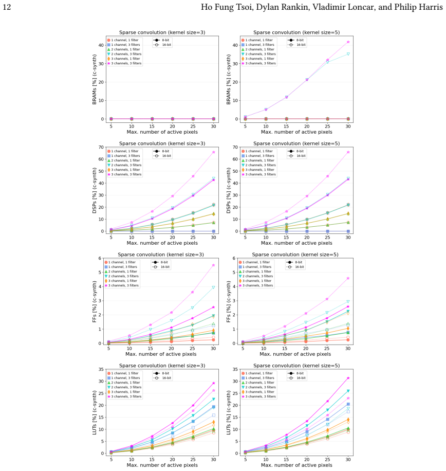
Summary. The paper presents SparsePixels, an FPGA framework for sparse 2D convolution. The key idea is to retain at most N_max_active pixels from a large, spatially sparse input using a fixed, row-major reduction tree, then perform all subsequent convolution, activation, pooling, and flattening operations on compact sparse arrays with a fixed active set. This makes inference latency independent of input sparsity and bounded by the pixel budget. The authors implement the sparse layers in HLS, provide a Python library for quantization-aware training, and release the code. They compare sparse CNNs against standard hls4ml stream-I/O CNNs on MNIST, MicroBooNE neutrino images, and LHC jet tagging, reporting large speedups on an Alveo FPGA. For MicroBooNE, the sparse-large model achieves 133 cycles (0.665 us) versus 9733 cycles (48.665 us) for the standard CNN, a factor-73 speedup, with ROC AUC 0.927 versus 0.943. The central claim is that this speed-accuracy trade-off is practically useful for low-latency scientific data readout.
Significance. If the reported accuracy results are robust, this is a useful and timely contribution. The paper provides detailed pseudocode for all sparse layers, a public code release, careful latency and resource scaling studies, and concrete FPGA measurements on realistic high-energy physics datasets. The constant-latency property enforced by N_max_active is an important practical feature for trigger systems with hard latency bounds. The sparse-convolution formulation is well grounded in prior submanifold sparse convolution work, and the FPGA implementation is nontrivial. However, the significance is currently conditional: the headline "<2% AUC drop" is established for a single crop/vertex distribution and a single baseline, and the row-major active-pixel truncation is not tested for spatial-order sensitivity. If the requested robustness experiments are added and the accuracy differences are confirmed with uncertainty quantification, the paper would be a strong systems contribution.
major comments (3)
- [Secs. 3.2.1 and 4.2.1, Algorithm 1, Fig. 10] The row-major truncation of active pixels is load-bearing for the main accuracy claim but is not tested for robustness to input translation or alternative selection order. Algorithm 1 retains the first N_max_active active pixels in row-major order, and for MicroBooNE sparse-large this is only 20 of 3969 pixels. The paper itself shows in Fig. 10 that row-major truncation can change a digit 9 into a 0 at small N_max_active. Since the motivating LArTPC application must handle neutrino interactions occurring anywhere in the detector, the reported 0.927 versus 0.943 AUC in Table 1 may depend on the particular crop/vertex placement in the signal windows. I request an ablation that translates or re-crops MicroBooNE signal windows and/or uses a different active-pixel ordering (e.g., sorted by intensity, top-k by feature value) and reports AUC versus N_max_active for each condition. Without this,
- [Sec. 4.2.2 and Table 1] All accuracy/AUC values are single-run point estimates without repeated-seed variance. The differences being cited, such as MicroBooNE 8-bit sparse-large AUC 0.927 versus standard 0.943, are small enough that seed-induced variability could change the conclusion. Additionally, N_max_active is selected from a scan, and the reported numbers are the favorable operating points; while this is a standard hyperparameter choice, the selection should be based on validation and the test-set result should be reported with mean and standard deviation over multiple training runs. Please add this information, at least for the three datasets in Table 1.
- [Sec. 4.2.2] The standard and sparse CNNs are synthesized with different HLS toolchains: standard CNNs with Vivado HLS 2020.1 and sparse CNNs with Vitis HLS 2023.1. Since the headline speedup is a ratio of latencies measured from these two toolchains, the comparison would be cleaner if both designs were synthesized with the same tool version (or if the authors justify that the difference is immaterial for the stream-I/O versus parallel-I/O contrast). At minimum, the paper should state whether this choice was driven by hls4ml stability and whether any cross-tool latency differences were observed for the same design.
minor comments (4)
- [Sec. 4.2.1] Typos: 'boarders' should be 'borders' in the MNIST and jet preprocessing descriptions; 'gloun' should be 'gluon' in the jet tagging dataset description.
- [Table 1 and figure captions] 'Latancy' is misspelled 'Latency' in the Table 1 caption and in Figs. 16, 17, 21, and 22. Also, 'Fig. 17 Fig. 22' in Sec. 4.2.3 should be 'Fig. 17 and Fig. 22'.
- [Algorithm 2, line 21] The condition 'if pixel p_out is padded' is not defined in the algorithm or in the surrounding text. Since the convolution uses 'same' padding and the active set is fixed, it should be clarified what 'padded' means for a sparse output pixel and how the HLS implementation detects it.
- [Sec. 4.2.1, MicroBooNE preprocessing] Please state explicitly whether the 256x512 signal windows are centered or aligned on the neutrino vertex or are cropped at fixed coordinates. This detail is important for interpreting the row-major truncation behavior in the accuracy results.
Circularity Check
No significant circularity: N_max_active is an openly scanned hyperparameter; speedups and accuracy are direct benchmarks on public data.
full rationale
The paper's central claimed result—a x73 FPGA speedup with <2% AUC drop on MicroBooNE—is not a prediction obtained from fitted parameters. SparsePixels' core sparsity-preserving convolution is defined in Sec. 3.1 and explicitly attributed to external prior work [32] (Graham et al.), not to a self-cited uniqueness theorem or ansatz. N_max_active is explicitly called a hyperparameter in Sec. 3.2.1, and Sec. 4.2.1 says an N_max_active scan is necessary to balance accuracy and hardware cost; Table 1 reports measured results for the scanned values {8,12,16,20}, so accuracy is not a fitted quantity renamed as a prediction. The constant-runtime property is a design guarantee following from fixed sparse-array sizes, not an empirical discovery derived from data. The hls4ml baseline is measured with released code, and the paper's self-citations (e.g., hls4ml, FastML team) support tooling and related work rather than bearing the load of the trade-off claim. The acknowledged limitation that row-major truncation can discard discriminative pixels (Sec. 4.2.1, Fig. 10) is a correctness/robustness concern about order dependence, not a circular step: no equation in the paper reduces to its own input by construction. Overall, the derivation chain is self-contained as an engineering benchmark.
Axiom & Free-Parameter Ledger
free parameters (4)
- N_max_active =
8, 12, 16, 20 (per dataset/model)
- Active-pixel threshold(s) =
MNIST 0.4; MicroBooNE 700 (denoised); LHC jet 0.003 after normalization
- Input preprocessing / image shaping =
MNIST 48x48 after pool-3 and inflation; MicroBooNE 63x63 by summing 256x512 windows; jet crop to 56x56 with radial infla
- Total bit-width (quantization) =
8 or 16 bits
axioms (4)
- domain assumption Thresholded active pixels carry the discriminative information; inactive pixels can be discarded without material accuracy loss.
- domain assumption Submanifold sparsity preservation -- an output pixel is active iff the corresponding input pixel is active -- is expressive enough for classification after stacking layers/kernels.
- domain assumption Row-major top-N_max truncation of active pixels is an acceptable information-loss mechanism for sparse images.
- domain assumption HLS synthesis (Vitis/Vivado) correctly models FPGA latency and resource usage at 200 MHz; logic-synthesis numbers for full models are reliable.
read the original abstract
Inference of standard convolutional neural networks (CNNs) on FPGAs often incurs high latency and a long initiation interval due to the deep nested loops required to densely convolve every input pixel regardless of its feature value. However, input features can be spatially sparse in some image data, where semantic information may occupy only a small fraction of the pixels and most computation would be wasted on empty regions. In this work, we introduce SparsePixels, a framework that implements sparse convolution on FPGAs by selectively retaining and computing on a small subset of active pixels while ignoring the rest. Because computation always runs over a single pre-specified pixel budget, the inference latency is independent of the input sparsity and is constant at runtime. We show that, for identifying neutrino interactions in naturally sparse LArTPC images with 4k pixels, a standard CNN with a compact size of 4k parameters incurs an inference latency of 48.665 $\mu$s on an FPGA, whereas a sparse CNN of the same base architecture, computing on less than 1% of the input pixels, achieves a $\times 73$ speedup to 0.665 $\mu$s with resource utilization well within on-chip budgets, trading only a small percent-level performance loss. This work aims to benefit future algorithm development for efficient data readout in modern experiments with latency requirements of microseconds or below.
Figures




Reference graph
Works this paper leans on
-
[1]
Georges Aad et al . 2020. Operation of the ATLAS trigger system in Run 2.JINST15, 10 (2020), P10004. arXiv:2007.12539 [physics.ins-det] doi:10.1088/1748-0221/15/10/P10004
Pith/arXiv arXiv 2020
-
[2]
Thea Aarrestad et al . 2021. Fast convolutional neural networks on FPGAs with hls4ml.Mach. Learn. Sci. Tech.2, 4 (2021), 045015. arXiv:2101.05108 [cs.LG] doi:10.1088/2632-2153/ac0ea1
Pith/arXiv arXiv 2021
-
[3]
Thea Aarrestad et al. 2022. The Dark Machines Anomaly Score Challenge: Benchmark Data and Model Independent Event Classification for the Large Hadron Collider.SciPost Phys.12, 1 (2022), 043. arXiv:2105.14027 [hep-ph] doi:10.21468/SciPostPhys.12.1.043
Pith/arXiv arXiv 2022
- [4]
-
[5]
2022.MicroBooNE BNB Electron Neutrino Overlay Sample (With Wire Info)
Polina Abratenko et al. 2022.MicroBooNE BNB Electron Neutrino Overlay Sample (With Wire Info). doi:10.5281/zenodo.7262140
-
[6]
2022.MicroBooNE BNB Inclusive Overlay Sample (With Wire Info)
Polina Abratenko et al. 2022.MicroBooNE BNB Inclusive Overlay Sample (With Wire Info). doi:10.5281/zenodo.7262009
-
[7]
R. Acciarri et al. 2017. Convolutional Neural Networks Applied to Neutrino Events in a Liquid Argon Time Projection Chamber.JINST12, 03 (2017), P03011. arXiv:1611.05531 [physics.ins-det] doi:10.1088/1748-0221/12/03/P03011
Pith/arXiv arXiv 2017
-
[8]
R. Acciarri et al. 2017. Design and Construction of the MicroBooNE Detector.JINST12, 02 (2017), P02017. arXiv:1612.05824 [physics.ins-det] doi:10.1088/1748-0221/12/02/P02017
Pith/arXiv arXiv 2017
-
[9]
AMD. 2023. Vitis Libraries (2023.1). https://docs.amd.com/r/2023.1-English/Vitis_Libraries/index.html
2023
-
[10]
A. Aurisano, A. Radovic, D. Rocco, A. Himmel, M. D. Messier, E. Niner, G. Pawloski, F. Psihas, A. Sousa, and P. Vahle. 2016. A Convolutional Neural Network Neutrino Event Classifier.JINST11, 09 (2016), P09001. arXiv:1604.01444 [hep-ex] doi:10.1088/1748-0221/11/09/P09001
Pith/arXiv arXiv 2016
-
[11]
Michaela Blott, Thomas B Preußer, Nicholas J Fraser, Giulio Gambardella, Kenneth O’brien, Yaman Umuroglu, Miriam Leeser, and Kees Vissers. 2018. FINN-R: An end-to-end deep-learning framework for fast exploration of quantized neural networks.ACM Transactions on Reconfigurable Technology and Systems (TRETS)11, 3 (2018), 1–23
2018
-
[12]
Anja Butter et al . 2019. The Machine Learning landscape of top taggers.SciPost Phys.7 (2019), 014. arXiv:1902.09914 [hep-ph] doi:10.21468/ SciPostPhys.7.1.014
Pith/arXiv arXiv 2019
-
[13]
Matteo Cacciari, Gavin P. Salam, and Gregory Soyez. 2008. The anti-𝑘𝑡 jet clustering algorithm.JHEP04 (2008), 063. arXiv:0802.1189 [hep-ph] doi:10.1088/1126-6708/2008/04/063
Pith/arXiv arXiv 2008
-
[14]
François Chollet et al. 2015. Keras. https://keras.io
2015
-
[15]
Christopher Choy, JunYoung Gwak, and Silvio Savarese. 2019. 4D Spatio-Temporal ConvNets: Minkowski Convolutional Neural Networks. In Proceedings of the IEEE Conference on Computer Vision and Pattern Recognition. 3075–3084
2019
-
[16]
Seokju Chung, Jack Cleeve, Akshay Malige, Georgia Karagiorgi, Lino Gerlach, Adrian A. Pol, and Isobel Ojalvo. 2025. Real-time Anomaly Detection for Liquid Argon Time Projection Chambers. (9 2025). arXiv:2509.21817 [hep-ex]
Pith/arXiv arXiv 2025
-
[17]
Andrea Coccaro, Francesco Armando Di Bello, Stefano Giagu, Lucrezia Rambelli, and Nicola Stocchetti. 2023. Fast neural network inference on FPGAs for triggering on long-lived particles at colliders.Mach. Learn. Sci. Tech.4, 4 (2023), 045040. arXiv:2307.05152 [hep-ex] doi:10.1088/2632-2153/ad087a
Pith/arXiv arXiv 2023
-
[18]
Claudionor N. Coelho, Aki Kuusela, Shan Li, Hao Zhuang, Thea Aarrestad, Vladimir Loncar, Jennifer Ngadiuba, Maurizio Pierini, Adrian Alan Pol, and Sioni Summers. 2021. Automatic heterogeneous quantization of deep neural networks for low-latency inference on the edge for particle detectors.Nature Mach. Intell.3 (2021), 675–686. arXiv:2006.10159 [physics.in...
Pith/arXiv arXiv 2021
-
[19]
ATLAS Collaboration. 2018. Technical Design Report for the Phase-II Upgrade of the ATLAS TDAQ System.ATLAS Technical Design Report CERN-LHCC-2017-020, ATLAS-TDR-029 (2018). doi:10.17181/CERN.2LBB.4IAL
-
[20]
CMS Collaboration. 2020. The Phase-2 Upgrade of the CMS Level-1 Trigger.CMS Technical Design ReportCERN-LHCC-2020-004, CMS-TDR-021 (2020)
2020
-
[21]
CMS Collaboration. 2023. Level-1 Trigger Calorimeter Image Convolutional Anomaly Detection Algorithm. (2023). https://cds.cern.ch/record/2879816
arXiv 2023
-
[22]
CMS Collaboration. 2024. Model-Independent Real-Time Anomaly Detection at the CMS Level-1 Calorimeter Trigger with CICADA. (2024). https://cds.cern.ch/record/2917884
arXiv 2024
-
[23]
Luke de Oliveira, Michael Kagan, Lester Mackey, Benjamin Nachman, and Ariel Schwartzman. 2016. Jet-images — deep learning edition.JHEP07 (2016), 069. arXiv:1511.05190 [hep-ph] doi:10.1007/JHEP07(2016)069
Pith/arXiv arXiv 2016
-
[24]
Laura Dominé and Kazuhiro Terao. 2020. Scalable deep convolutional neural networks for sparse, locally dense liquid argon time projection chamber data.Phys. Rev. D102, 1 (2020), 012005. arXiv:1903.05663 [hep-ex] doi:10.1103/PhysRevD.102.012005
Pith/arXiv arXiv 2020
-
[25]
Javier Duarte et al . 2018. Fast inference of deep neural networks in FPGAs for particle physics.JINST13, 07 (2018), P07027. arXiv:1804.06913 [physics.ins-det] doi:10.1088/1748-0221/13/07/P07027
Pith/arXiv arXiv 2018
-
[26]
2025.fastmachinelearning/hls4ml
FastML Team. 2025.fastmachinelearning/hls4ml. doi:10.5281/zenodo.1201549
-
[27]
Simone Francescato et al. 2021. Model compression and simplification pipelines for fast deep neural network inference in FPGAs in HEP.Eur. Phys. J. C81, 11 (2021), 969. doi:10.1140/epjc/s10052-021-09770-w [Erratum: Eur.Phys.J.C 81, 1064 (2021)]
-
[28]
Abhijith Gandrakota. 2025. Realtime Anomaly Detection at the L1 Trigger of CMS Experiment.PoSICHEP2024 (2025), 1025. arXiv:2411.19506 [hep-ex] doi:10.22323/1.476.1025
Pith/arXiv arXiv 2025
-
[29]
Nicolò Ghielmetti et al. 2022. Real-time semantic segmentation on FPGAs for autonomous vehicles with hls4ml.Mach. Learn. Sci. Tech.(2022). arXiv:2205.07690 [cs.CV] doi:10.1088/2632-2153/ac9cb5 Manuscript submitted to ACM SparsePixels: Efficient Convolution for Sparse Data on FPGAs 21
Pith/arXiv arXiv 2022
-
[30]
Ekaterina Govorkova et al. 2022. Autoencoders on field-programmable gate arrays for real-time, unsupervised new physics detection at 40 MHz at the Large Hadron Collider.Nature Mach. Intell.4 (2022), 154–161. arXiv:2108.03986 [physics.ins-det] doi:10.1038/s42256-022-00441-3
Pith/arXiv arXiv 2022
-
[31]
Ben Graham. 2015. Sparse 3D convolutional neural networks. arXiv:1505.02890 [cs.CV] https://arxiv.org/abs/1505.02890
Pith/arXiv arXiv 2015
-
[32]
Benjamin Graham, Martin Engelcke, and Laurens van der Maaten. 2018. 3D Semantic Segmentation with Submanifold Sparse Convolutional Networks. In2018 IEEE/CVF Conference on Computer Vision and Pattern Recognition (CVPR). 9224–9232. arXiv:1711.10275 doi:10.1109/CVPR.2018.00961
Pith/arXiv arXiv 2018
-
[33]
Khoda, Scott Hauck, Shih-Chieh Hsu, Ekaterina Govorkova, Philip Harris, Vladimir Loncar, and Eric A
Zhixing Jiang, Dennis Yin, Yihui Chen, Elham E. Khoda, Scott Hauck, Shih-Chieh Hsu, Ekaterina Govorkova, Philip Harris, Vladimir Loncar, and Eric A. Moreno. 2025. Low latency transformer inference on FPGAs for physics applications with hls4ml.JINST20, 04 (2025), P04014. arXiv:2409.05207 [cs.LG] doi:10.1088/1748-0221/20/04/P04014
Pith/arXiv arXiv 2025
-
[34]
Gregor Kasieczka et al. 2021. The LHC Olympics 2020 a community challenge for anomaly detection in high energy physics.Rept. Prog. Phys.84, 12 (2021), 124201. arXiv:2101.08320 [hep-ph] doi:10.1088/1361-6633/ac36b9
Pith/arXiv arXiv 2021
-
[35]
Gregor Kasieczka, Tilman Plehn, Michael Russell, and Torben Schell. 2017. Deep-learning Top Taggers or The End of QCD?JHEP05 (2017), 006. arXiv:1701.08784 [hep-ph] doi:10.1007/JHEP05(2017)006
Pith/arXiv arXiv 2017
-
[36]
Elham E. Khoda et al. 2023. Ultra-low latency recurrent neural network inference on FPGAs for physics applications with hls4ml.Mach. Learn. Sci. Tech.4, 2 (2023), 025004. arXiv:2207.00559 [cs.LG] doi:10.1088/2632-2153/acc0d7
Pith/arXiv arXiv 2023
-
[37]
Diederik P. Kingma and Jimmy Ba. 2017. Adam: A Method for Stochastic Optimization. arXiv:1412.6980 [cs.LG]
Pith/arXiv arXiv 2017
-
[38]
Yann LeCun, Yoshua Bengio, and Geoffrey Hinton. 2015. Deep learning.Nature521 (2015), 436–444. doi:10.1038/nature14539
-
[39]
Yann LeCun and Corinna Cortes. 2010. MNIST handwritten digit database. http://yann.lecun.com/exdb/mnist/. (2010). http://yann.lecun.com/exdb/ mnist/
2010
-
[40]
Baoyuan Liu, Min Wang, Hassan Foroosh, Marshall Tappen, and Marianna Penksy. 2015. Sparse Convolutional Neural Networks. In2015 IEEE Conference on Computer Vision and Pattern Recognition (CVPR). 806–814. doi:10.1109/CVPR.2015.7298681
arXiv 2015
-
[41]
Liqiang Lu, Jiaming Xie, Ruirui Huang, Jiansong Zhang, Wei Lin, and Yun Liang. 2019. An Efficient Hardware Accelerator for Sparse Convolutional Neural Networks on FPGAs. In2019 IEEE 27th Annual International Symposium on Field-Programmable Custom Computing Machines (FCCM). 17–25. doi:10.1109/FCCM.2019.00013
arXiv 2019
-
[42]
Leandro Maglianella, Lorenzo Nicoletti, Stefano Giagu, Christian Napoli, and Simone Scardapane. 2023. Convergent Approaches to AI Explainability for HEP Muonic Particles Pattern Recognition.Comput. Softw. Big Sci.7, 1 (2023), 8. doi:10.1007/s41781-023-00102-z
-
[43]
Eric A. Moreno, Olmo Cerri, Javier M. Duarte, Harvey B. Newman, Thong Q. Nguyen, Avikar Periwal, Maurizio Pierini, Aidana Serikova, Maria Spiropulu, and Jean-Roch Vlimant. 2020. JEDI-net: a jet identification algorithm based on interaction networks.Eur. Phys. J. C80, 1 (2020), 58. arXiv:1908.05318 [hep-ex] doi:10.1140/epjc/s10052-020-7608-4
Pith/arXiv arXiv 2020
-
[44]
Adam Paszke, Sam Gross, Francisco Massa, Gal Lerer, James Bradbury, Gregory Chanan, Trevor Killeen, Zeming Lin, Naresh Gimelshein, Luca Antiga, et al. 2019. PyTorch: An Imperative Style, High-Performance Deep Learning Library.Advances in Neural Information Processing Systems32 (2019)
2019
-
[45]
2020.HLS4ML LHC Jet dataset (150 particles)
Maurizio Pierini, Javier Mauricio Duarte, Nhan Tran, and Marat Freytsis. 2020.HLS4ML LHC Jet dataset (150 particles). doi:10.5281/zenodo.3602260
-
[46]
Adrian Alan Pol et al. 2021. Jet Single Shot Detection.EPJ Web Conf.251 (2021), 04027. arXiv:2105.05785 [hep-ex] doi:10.1051/epjconf/202125104027
Pith/arXiv arXiv 2021
-
[47]
Albert M Sirunyan et al. 2020. Performance of the CMS Level-1 trigger in proton-proton collisions at√𝑠= 13 TeV.JINST15, 10 (2020), P10017. arXiv:2006.10165 [hep-ex] doi:10.1088/1748-0221/15/10/P10017
Pith/arXiv arXiv 2020
-
[48]
Sioni Summers et al . 2020. Fast inference of Boosted Decision Trees in FPGAs for particle physics.JINST15, 05 (2020), P05026. arXiv:2002.02534 [physics.comp-ph] doi:10.1088/1748-0221/15/05/P05026
Pith/arXiv arXiv 2020
-
[49]
Arrestad, Vladimir Loncar, Jennifer Ngadiuba, and Maria Spiropulu
Chang Sun, Thea K. Arrestad, Vladimir Loncar, Jennifer Ngadiuba, and Maria Spiropulu. 2024. Gradient-based Automatic Mixed Precision Quantization for Neural Networks On-Chip. (5 2024). arXiv:2405.00645 [cs.LG] doi:10.7907/hq8jd-rhg30
arXiv 2024
-
[50]
Haotian Tang, Zhijian Liu, Xiuyu Li, Yujun Lin, and Song Han. 2022. TorchSparse: Efficient Point Cloud Inference Engine. InConference on Machine Learning and Systems (MLSys)
2022
-
[51]
Haotian Tang, Shang Yang, Zhijian Liu, Ke Hong, Zhongming Yu, Xiuyu Li, Guohao Dai, Yu Wang, and Song Han. 2023. TorchSparse++: Efficient Training and Inference Framework for Sparse Convolution on GPUs. InIEEE/ACM International Symposium on Microarchitecture (MICRO)
2023
-
[52]
Naif Tarafdar, Giuseppe Di Guglielmo, Philip C. Harris, Jeffrey D. Krupa, Vladimir Loncar, Dylan S. Rankin, Nhan Tran, Zhenbin Wu, Qianfeng Clark Shen, and Paul Chow. 2022. AIgean: An Open Framework for Deploying Machine Learning on Heterogeneous Clusters.ACM Trans. Reconf. Tech. Syst.15, 3 (2022), 1–32. doi:10.1145/3482854
-
[53]
Ho Fung Tsoi, Vladimir Loncar, Sridhara Dasu, and Philip Harris. 2025. SymbolNet: neural symbolic regression with adaptive dynamic pruning for compression.Mach. Learn. Sci. Tech.6, 1 (2025), 015021. arXiv:2401.09949 [cs.LG] doi:10.1088/2632-2153/adaad8
Pith/arXiv arXiv 2025
-
[54]
Ho Fung Tsoi, Adrian Alan Pol, Vladimir Loncar, Ekaterina Govorkova, Miles Cranmer, Sridhara Dasu, Peter Elmer, Philip Harris, Isobel Ojalvo, and Maurizio Pierini. 2024. Symbolic Regression on FPGAs for Fast Machine Learning Inference.EPJ Web Conf.295 (2024), 09036. arXiv:2305.04099 [cs.LG] doi:10.1051/epjconf/202429509036
Pith/arXiv arXiv 2024
-
[55]
Fraser, Giulio Gambardella, Michaela Blott, Philip Leong, Magnus Jahre, and Kees Vissers
Yaman Umuroglu, Nicholas J. Fraser, Giulio Gambardella, Michaela Blott, Philip Leong, Magnus Jahre, and Kees Vissers. 2017. FINN: A Framework for Fast, Scalable Binarized Neural Network Inference. InProceedings of the 2017 ACM/SIGDA International Symposium on Field-Programmable Gate Arrays (FPGA ’17). ACM, 65–74
2017
-
[56]
Jure Vreča and Anton Biasizzo. 2025. Generating Direct Logic Circuit Implementations of Deeply Quantized Neural Networks Using Chisel4ml. Electronics14, 5 (2025). doi:10.3390/electronics14050849 Manuscript submitted to ACM 22 Ho Fung Tsoi, Dylan Rankin, Vladimir Loncar, and Philip Harris
-
[57]
Derek Weitzel, Ashton Graves, Sam Albin, Huijun Zhu, Frank Wuerthwein, Mahidhar Tatineni, Dmitry Mishin, Elham Khoda, Mohammad Sada, Larry Smarr, Thomas DeFanti, and John Graham. 2025. The National Research Platform: Stretched, Multi-Tenant, Scientific Kubernetes Cluster. InPractice and Experience in Advanced Research Computing 2025: The Power of Collabor...
arXiv 2025
-
[58]
Xilinx. 2020. Vivado Design Suite User Guide: High-Level Synthesis. https://www.xilinx.com/support/documentation/sw_manuals/xilinx2020_1/ ug902-vivado-high-level-synthesis.pdf
2020
-
[59]
Yan Yan, Yuxing Mao, and Bo Li. 2018. SECOND: Sparsely Embedded Convolutional Detection.Sensors18, 10 (2018). doi:10.3390/s18103337
-
[60]
Chaoyang Zhu, Kejie Huang, Shuyuan Yang, Ziqi Zhu, Hejia Zhang, and Haibin Shen. 2020. An Efficient Hardware Accelerator for Structured Sparse Convolutional Neural Networks on FPGAs.IEEE Trans. Very Large Scale Integr. Syst.28, 9 (Sept. 2020), 1953–1965. doi:10.1109/TVLSI.2020.3002779
arXiv 2020
-
[61]
I. Zurbano Fernandez et al. 2020. High-Luminosity Large Hadron Collider (HL-LHC): Technical design report. 10/2020 (12 2020). doi:10.23731/CYRM- 2020-0010 Manuscript submitted to ACM SparsePixels: Efficient Convolution for Sparse Data on FPGAs 23 Algorithm 3:Sparse Activation in HLS Inputs :sparse feature array𝑎 in feat[0..𝑁 max active·𝐶−1] Outputs :spars...
doi:10.23731/cyrm- 2020
discussion (0)
Sign in with ORCID, Apple, or X to comment. Anyone can read and Pith papers without signing in.