REVIEW 2 major objections 2 minor 24 references
Semiparametrically Efficient Inference for Kernel Measures of Noise Heterogeneity
T0 review · 2 major / 2 minor · reviewed 2026-06-29 · grok-4.3
Pith's one-line read A Hilbert-valued one-step estimator achieves semiparametric efficiency for kernel measures of noise heterogeneity after machine learning regression.
desk verdict The paper's one-step Hilbert-valued estimator for the kernel covariance operator between covariates and residuals offers a targeted bias correction after ML regression, but the efficiency claim rests on first-stage rates that need explicit checks in the operator setting. read the letter →
The pith
A machine-rendered reading of the paper's core claim, the machinery that carries it, and where it could break.
The reading
What carries the argument
Hilbert-valued one-step estimator of the kernel covariance operator between covariates and residuals, which removes first-stage bias from the machine learning estimator of the regression function.
What would settle it
Observing that the estimator does not achieve the efficiency bound or that tests lose calibration when the first-stage estimator violates the rate conditions would falsify the central claim.
Extended reading notes
Core claim
The central claim is that the novel Hilbert-valued one-step estimator of the kernel covariance operator between covariates and residuals yields bootstrap-calibrated tests for residual independence and goodness of fit in additive noise models, while also providing asymptotically efficient confidence intervals for the kernel dependence measure under noise heterogeneity.
Load-bearing premise
The first-stage machine learning estimator of the regression function must satisfy the necessary rate and regularity conditions for the one-step correction to remove bias.
Editorial extensions
If this is right
- The estimator supports bootstrap-calibrated tests for residual independence in additive noise models.
- It provides asymptotically efficient confidence intervals for the kernel dependence measure.
- The framework extends to settings with additional covariates for inference on distributional heterogeneity across treatment groups.
- Simulations demonstrate improved calibration and power over naive plug-in residual methods.
Reading between the lines
- The method could be applied to other first-stage machine learning tasks where residual analysis is needed for dependence testing.
- It opens possibilities for semiparametric inference in more complex models beyond additive noise.
- Practitioners might use this to validate assumptions in causal models relying on residual independence.
Editorial analysis
A structured set of objections, weighed in public.
Referee Report
Summary. The manuscript develops a semiparametrically efficient Hilbert-valued one-step estimator for the kernel covariance operator between covariates and residuals in additive noise models. It claims this corrects first-stage bias from machine learning regression estimators, yielding bootstrap-calibrated tests for residual independence and goodness-of-fit, asymptotically efficient confidence intervals for the kernel dependence measure under noise heterogeneity, and extensions to inference on distributional heterogeneity across treatment groups with additional covariates. Simulations are reported to show improved calibration and power relative to naive plug-in methods.
Significance. If the efficiency and bootstrap validity claims hold under verifiable conditions, the framework would enable robust post-ML inference on noise heterogeneity and residual dependence, addressing a practical limitation in nonparametric and high-dimensional regression analysis. The operator-valued one-step correction and treatment-group extension represent a targeted contribution to semiparametric methods for dependence measures.
major comments (2)
- [Theoretical construction of the one-step estimator] The central efficiency claim for the Hilbert-valued one-step estimator rests on the first-stage ML regression estimator satisfying rate conditions (typically faster than n^{-1/4} convergence in suitable norms) and regularity (e.g., Donsker-type) sufficient for the correction term to eliminate bias in the operator setting. The construction (as described in the abstract and theoretical development) invokes these implicitly without explicit sufficient conditions or verification tailored to the operator norm, which is load-bearing for the semiparametric efficiency and bootstrap calibration results.
- [Simulations] Table or simulation results section: the reported gains in calibration and power are presented without a detailed description of the simulation design (exact ML nuisance estimators, sample sizes, dimension settings, and bootstrap implementation), preventing assessment of whether the empirical evidence supports the efficiency claims under the paper's own regularity conditions.
minor comments (2)
- [Notation and definitions] Clarify notation for the kernel covariance operator, the precise Hilbert space, and the form of the one-step correction term to improve readability for readers unfamiliar with operator-valued semiparametrics.
- [Assumptions] Add explicit statements of all technical assumptions (including on the kernel and the nuisance estimator) in a dedicated assumptions subsection rather than scattering them.
Simulated Author's Rebuttal
We thank the referee for the constructive and detailed comments, which help clarify the presentation of our theoretical results and empirical evidence. We address each major comment below and will incorporate the suggested changes in the revised manuscript.
read point-by-point responses
-
Referee: [Theoretical construction of the one-step estimator] The central efficiency claim for the Hilbert-valued one-step estimator rests on the first-stage ML regression estimator satisfying rate conditions (typically faster than n^{-1/4} convergence in suitable norms) and regularity (e.g., Donsker-type) sufficient for the correction term to eliminate bias in the operator setting. The construction (as described in the abstract and theoretical development) invokes these implicitly without explicit sufficient conditions or verification tailored to the operator norm, which is load-bearing for the semiparametric efficiency and bootstrap calibration results.
Authors: We agree that explicit statement of the conditions is important for the operator-valued setting. The current development relies on standard semiparametric rate and regularity assumptions for the first-stage estimators, but we will add a new subsection in the theoretical section that explicitly lists the required conditions, including n^{-1/4} rates in the appropriate operator norm, Donsker-type classes adapted to the Hilbert space, and references to supporting results from the semiparametric literature on infinite-dimensional functionals. This will make the load-bearing assumptions transparent and verifiable. revision: yes
-
Referee: [Simulations] Table or simulation results section: the reported gains in calibration and power are presented without a detailed description of the simulation design (exact ML nuisance estimators, sample sizes, dimension settings, and bootstrap implementation), preventing assessment of whether the empirical evidence supports the efficiency claims under the paper's own regularity conditions.
Authors: We concur that fuller documentation of the simulation design is needed. In the revision we will expand the relevant section to specify the exact machine learning procedures and hyperparameters used for the nuisance estimators, the full range of sample sizes and covariate dimensions, the precise bootstrap implementation (including number of replicates and resampling scheme), and how these choices satisfy the paper's regularity conditions. This will enable readers to assess alignment between theory and experiments. revision: yes
Circularity Check
No significant circularity; standard one-step semiparametric construction
full rationale
The paper develops a Hilbert-valued one-step estimator of the kernel covariance operator between covariates and residuals. The claimed semiparametric efficiency and bootstrap calibration follow from applying a standard one-step bias-correction term under external nuisance rate conditions (n^{-1/4} or faster, Donsker-type), which are not derived from or equivalent to the paper's own fitted quantities or self-citations. No self-definitional steps, fitted inputs renamed as predictions, or load-bearing self-citation chains appear in the abstract or described framework. The construction is self-contained against external semiparametric benchmarks.
Assumptions & free parameters
assumptions (1)
- domain assumption The regression function belongs to a class allowing consistent estimation at rates sufficient for the one-step correction to achieve efficiency.
Cite this review
Pith. "Pith review of Semiparametrically Efficient Inference for Kernel Measures of Noise Heterogeneity." pith.science (2026). https://pith.science/paper/RI4TSYPD
@misc{pith2026260527526,
  author       = {Pith},
  title        = {Pith review of: Semiparametrically Efficient Inference for Kernel Measures of Noise Heterogeneity},
  year         = {2026},
  howpublished = {\url{https://pith.science/paper/RI4TSYPD}},
  note         = {Machine review of arXiv:2605.27526}
}
read the original abstract
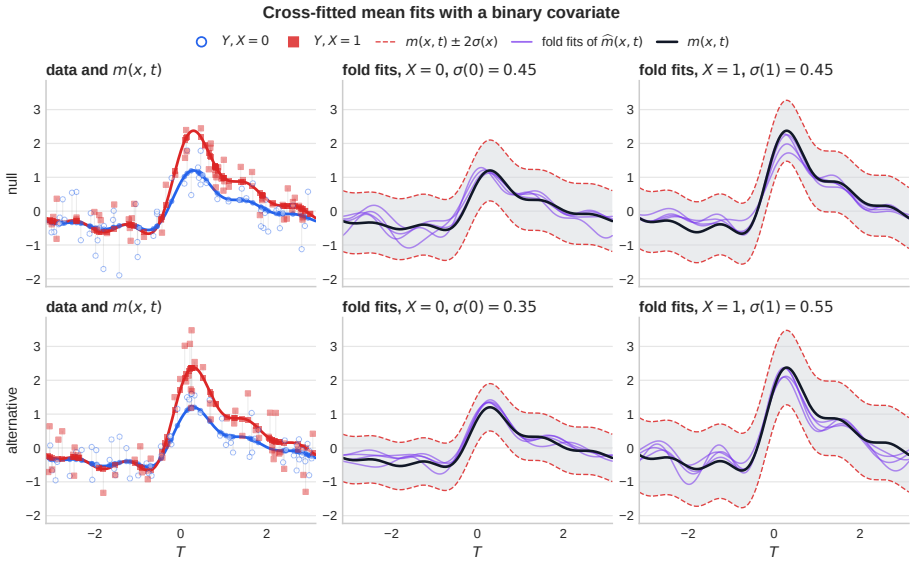
We develop semiparametrically efficient inference for kernel measures of noise heterogeneity in additive noise models. In many applications, the regression function is estimated using flexible machine learning methods. Downstream procedures based on the resulting residuals can then inherit first-stage bias: regression error may induce spurious dependence between covariates and residuals, invalidating the assumptions needed for standard analysis. We construct a novel Hilbert-valued one-step estimator of the kernel covariance operator between covariates and residuals. Our estimator yields bootstrap-calibrated tests for residual independence and goodness of fit in additive noise models, while also providing asymptotically efficient confidence intervals for the kernel dependence measure under noise heterogeneity. The framework extends to settings with additional covariates, enabling inference on distributional heterogeneity of residual noise across treatment groups. Simulations show improved calibration and power relative to naive plug-in residual methods.
Figures


Figures from the paper (15 more)




Reference graph
Works this paper leans on
-
[1]
Sinkhorn Treatment Effects: A Causal Optimal Transport Measure
Web. Medha Agarwal and Alex Luedtke. Sinkhorn treatment effects: A causal optimal transport measure. arXiv preprint arXiv:2605.08485,
-
[2]
A simpler condition for consistency of a kernel independence test
Arthur Gretton. A simpler condition for consistency of a kernel independence test.arXiv preprint arXiv:1501.06103,
-
[3]
On the hardness of conditional independence testing in practice.arXiv preprint arXiv:2512.14000,
Zheng He, Roman Pogodin, Yazhe Li, Namrata Deka, Arthur Gretton, and Danica J Suther- land. On the hardness of conditional independence testing in practice.arXiv preprint arXiv:2512.14000,
-
[4]
URLhttps://doi.org/10.1201/9780203734520
doi: 10.1201/ 9780203734520. URLhttps://doi.org/10.1201/9780203734520. Yazhe Li, Roman Pogodin, Danica J Sutherland, and Arthur Gretton. Self-supervised learning with kernel dependence maximization.Advances in Neural Information Processing Systems, 34:15543–15556,
-
[5]
URLhttps://par.nsf.gov/biblio/10649160
doi: 10.1093/jrsssb/qkaf052. URLhttps://par.nsf.gov/biblio/10649160. Alex Luedtke and Incheoul Chung. One-step estimation of differentiable Hilbert-valued parameters. The Annals of Statistics, 52(4):1534 – 1563,
-
[6]
URLhttps: //doi.org/10.1214/24-AOS2403
doi: 10.1214/24-AOS2403. URLhttps: //doi.org/10.1214/24-AOS2403. Alex Luedtke, Marco Carone, and Mark J van der Laan. An omnibus non-parametric test of equality in distribution for unknown functions.Journal of the Royal Statistical Society Series B: Statistical Methodology, 81(1):75–99,
-
[7]
Inference on Variable Importance for Treatment Effect Heterogeneity: Shapley Values and Beyond
Pawel Morzywolek, Peter B Gilbert, and Alex Luedtke. Inference on local variable importance measures for heterogeneous treatment effects.arXiv preprint arXiv:2510.18843,
-
[8]
Roman Pogodin, Antonin Schrab, Yazhe Li, Danica J Sutherland, and Arthur Gretton
doi: 10.15496/publikation-1672. Roman Pogodin, Antonin Schrab, Yazhe Li, Danica J Sutherland, and Arthur Gretton. Practical kernel tests of conditional independence.arXiv preprint arXiv:2402.13196,
Show all 24 references
-
[9]
6 Guide to appendix In this section, we provide a guide to the contents of the appendix. At the top of each section, we provide a table listing the notation used in that section, with the exception of Section 7, where we provide a table for notation used across the paper. Samp...
2024
-
[10]
In Section 13, we construct the data-adaptive diagnostic for the trustworthiness of the delta method introduced in Section 3.2
We then establish the consistency ofbσ2. In Section 13, we construct the data-adaptive diagnostic for the trustworthiness of the delta method introduced in Section 3.2. In Section 14, we provide a detailed introduction to statistical learning theory for vector-valued kernel ri...
2024
-
[11]
We have EP h eϕX,P (X)⊗eφξ,P (W, Y) i =E P [(φk(X)−E P [φk(X ′)])⊗(φ ξ,P (W, Y)−E P [φξ,P (W ′, Y ′)])] =E P [φk(X)⊗φ ξ,P (W, Y)]−E P [φk(X)]⊗E P [φξ,P (W, Y)]
Proof of Theorem 1 in the general setting where we drop Assumption 1.Following a standard con- vention in semiparametric statistical theory, we use the subscript0to denote any objects indexed by the true distributionP0. We have EP h eϕX,P (X)⊗eφξ,P (W, Y) i =E P [(φk(X)−E P [φ...
2025
-
[12]
We have f5(x, w, y) =f 6 f4(x, w, y) = (⟨f6, φk(x)⊗(∂ jφl)(h4(x, w, y))⟩Hkl)dy j=1 f3(x, w, y) =−(⟨f 6, φk(x)⊗(∂ jφl)(h4(x, w, y))⟩Hkl)dy j=1 f2(w) = (−E0 [⟨f6, φk(X)⊗(∂ jφl)(h4(X, W, Y))⟩ Hkl |W=w]) dy j=1 f1(x, w, y) = (−E0 [⟨f6, φk(X)⊗(∂ jφl)(h4(X, W, Y))⟩ Hkl |W=w]) dy j=1...
2025
-
[13]
The vector-valued KRR estimator has the representer form [Carmeli et al., 2006] bvj(w) = X t∈I2 ωj,t(w)Rj,t, where, writing Q = ( q(ws, wt))s,t∈I2 and qw = ( q(w, wt))t∈I2, ωj(w)⊤ = q⊤ w Q+ n 2 λj,nI −1 . Therefore, D bCi,bvj(w) E Hl = X t∈I2 ωj,t(w) ∂2,jl(bξi,bξt)− 2 n X s...
2006
-
[14]
Suppose thatbv−k j is the solution to a vector-valued kernel ridge regression with separable kernel [Li et al., 2024] Q(w1, w2) =q(w 1, w2)IdHl. Then it can be written as bv−k j (w) = X z′∈Z −k w−k j (z′, w)(∂jφl) bξ−k(z′) ,(7) wherez ′ = (w′, y′)and w−k j (z′, w) = Q−k + (n−n...
2024
-
[15]
bQV, bQU V-statistic and U-statistic center∥ˇΨn∥2 Hkl and its diagonal-term-free analogue
Gij Cross-fitted Gram entry⟨bD−k(i)(Oi),bD−k(j)(Oj)⟩Hkl, wherek(i)is the validation fold containingOi. bQV, bQU V-statistic and U-statistic center∥ˇΨn∥2 Hkl and its diagonal-term-free analogue. We build on Luedtke and Chung [2024, Section 4.2] to construct(1−α )-confidence set...
2024
-
[16]
ForΩ n = IdHkl, the confidence set is Cn(ζ) = h∈ H kl :∥ ˇΨn −h∥ 2 Hkl ≤ ζ n
If N (b) i denotes the number of timesOi appears in the bootstrap draw of its validation fold, then, forΩ n = IdHkl, ∥H(b) n ∥2 Hkl = 1 n nX i,j=1 {N (b) i −1}{N (b) j −1}G ij. ForΩ n = IdHkl, the confidence set is Cn(ζ) = h∈ H kl :∥ ˇΨn −h∥ 2 Hkl ≤ ζ n . Hence, by the reverse...
2000
-
[17]
The functional delta method therefore gives √n ∥ ˇΨn∥2 Hkl − ∥Ψ0∥2 Hkl ⇝2⟨Ψ 0,H⟩ Hkl
The mapT : Hkl →R defined by T (h) = ∥h∥2 Hkl is Fréchet differentiable at everyh∈ Hkl, with derivative ˙Th[u] = 2⟨h, u⟩Hkl . The functional delta method therefore gives √n ∥ ˇΨn∥2 Hkl − ∥Ψ0∥2 Hkl ⇝2⟨Ψ 0,H⟩ Hkl . SinceHis centered Gaussian and⟨Ψ 0,·⟩ Hkl is a continuous linear...
2009
-
[18]
In terms of asymptotic validity of the confidence sets, we can use whichever one we prefer. Since the positive bias ofbQV is not negligible in small sample settings, we suggest to center the delta-method confidence sets on bQU, which leads to empirically better performance. Ho...
2007
-
[19]
Improvements to the underlying raw independence test, such as Schrab et al
We use the classical permutation HSIC test [Gretton et al., 2007] as the plug-in baseline because it is the canonical residual-independence diagnostic in ANM experiments. Improvements to the underlying raw independence test, such as Schrab et al. [2022], are unrelated to the d...
2007
-
[20]
(EVD) (measures capacity ofHq) pS|W,σ,RConditional law of the labelSand constants in Eq
pExponent forµ i in Eq. (EVD) (measures capacity ofHq) pS|W,σ,RConditional law of the labelSand constants in Eq. (MOM). bvλ,evλ empirical vvKRR solution with estimated labels (i.e. plug-in regression function bm) in Eq. (14), empirical vvKRR with oracle labelsSj in Eq. (15). b...
2011
-
[21]
We first define the embeddingIw : Hq →L 2(PW,0), mapping a functionf∈ H q to its PW,0-equivalence class[ f]
and Steinwart and Scovel [2012]. We first define the embeddingIw : Hq →L 2(PW,0), mapping a functionf∈ H q to its PW,0-equivalence class[ f]. Since the kernelq is bounded, we know that this embedding is a well-defined Hilbert-Schmidt operator. Indeed, by [Steinwart and Scovel,...
2012
-
[22]
The α-interpolationspacedefinesaHilbertspace
is defined by [Hq]α := (X i∈I aiµα/2 i [ei] : (ai)i∈I ∈ℓ 2(I) ) ⊆L 2(PW,0), equipped with the inner product *X i∈I ai(µα/2 i [ei]), X i∈I bi(µα/2 i [ei]) + [Hq]α = X i∈I aibi, for (ai)i∈I ,(b i)i∈I ∈ℓ 2(I). The α-interpolationspacedefinesaHilbertspace. Moreover, µα/2 i [ei] i∈...
2006
-
[23]
and [Li et al., 2024, Section 2]. In the following, we will denoteG as the vRKHS induced by the kernel K:W × W → L(H l)with K(w, w ′) :=q(w, w ′) IdHl, w, w ′ ∈ W.(13) Theorem 5(vRKHS isomorphism).For every function F∈ G there exists a unique operator C∈S 2(Hq,H l)such that F ...
2024
-
[24]
The space[G] α is a Hilbert space equipped with the inner product ⟨F, G⟩α :=⟨C, L⟩ S2([Hq]α,Hl) (F, G∈[G] α), whereC=I −1(F), L=I −1(G)
The vector-valued interpolation space[G]α is defined as [G]α :=I(S 2([Hq]α,H l)) ={F|F=I(C), C∈S 2([Hq]α,H l)}. The space[G] α is a Hilbert space equipped with the inner product ⟨F, G⟩α :=⟨C, L⟩ S2([Hq]α,Hl) (F, G∈[G] α), whereC=I −1(F), L=I −1(G). Remark 4(Well-specified vers...
2007
Reviewed June 29, 2026 · model on record in the stance chip above.
Discussion (0). Sign in to comment.