REVIEW 2 major objections 5 minor 33 references
A multivariate time series alone can reveal the two-dimensional input–response plane through which a stable system transiently amplifies, and how close it sits to the amplification threshold.
Reviewed by Pith at T0; open to challenge. T0 means a machine referee read the full paper against a public rubric. the ladder, T0–T4 →
T0 review · deepseek-v4-flash
2026-08-02 01:07 UTC pith:RV2CA3OG
load-bearing objection The inference pipeline and synthetic ladder are genuinely useful, but the load-bearing threshold Kc(Δ) is asserted, not derived, and direct checks show it is not the actual amplification threshold—so R's advertised 'distance to threshold' semantics do not hold as stated. the 2 major comments →
Inferring Non-Normal Amplification Geometry from Multivariate Time Series
The pith
A machine-rendered reading of the paper's core claim, the machinery that carries it, and where it could break.
Core claim
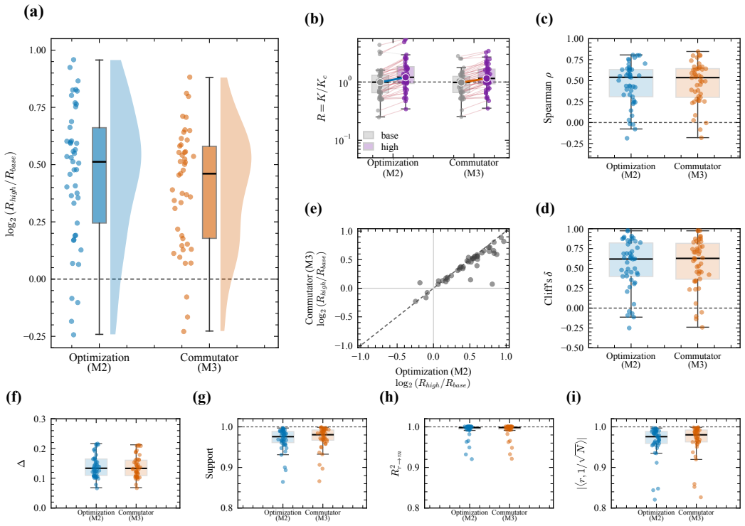
The central discovery is that the target of inference need not be the full N-dimensional operator: it can be a two-dimensional subspace that carries the input–response geometry. From a sliding window, the method estimates a local one-step linear map, then uses either an optimization that maximizes directed transverse coupling or a commutator construction to find the plane Q=[br,bn]. The projected 2x2 operator yields Δ, K, and R=K/Kc(Δ). The paper's synthetic evidence is that R and the plane are identifiable with a few percent of the N^2 samples needed for entrywise operator recovery, and that the extracted response direction aligns with burst activity in empirical recordings. The authors cla
What carries the argument
The central object is the projection of the fitted operator onto a two-dimensional orthonormal plane Q, giving Γ=Q^T F Q. The ratio R=K/Kc(Δ) normalizes the reduced non-normality index K by the threshold Kc(Δ)=[√(1−Δ²)/(1−√(1−Δ²))]^{1/2}, which the paper takes as the two-dimensional transient-amplification threshold. Two plane-extraction methods carry the argument: optimization-based directed-coupling extraction (M2), which searches for an orthonormal input/output pair maximizing transverse action, and commutator-based plane extraction (M3), which uses the symmetric commutator F F^T − F^T F to locate non-normal imbalance. The eigenbasis-SVD method (M1) is used as a fragile baseline.
Load-bearing premise
The entire reading of R=K/Kc(Δ) rests on the assertion that Kc(Δ) in Eq. (17) is the two-dimensional transient-amplification threshold, but the paper never derives it, its own Appendix B shows the exact threshold is scale-dependent, and a direct numerical check for the paper's canonical matrix fails, so R is a monotone relative diagnostic rather than an absolute distance to the true threshold.
What would settle it
Compute max_t ||F^t e_2|| for the paper's canonical matrix (A.2) with a=e^{−1}, b=e^{−2}: at the claimed threshold Kc=2.80 the norm peaks around 0.67, below 1, so no transient amplification occurs where the paper says R=1; any single (a,b) exhibiting the same mismatch settles that Kc is not the threshold.
If this is right
- Reduced geometry diagnostics can be tracked in moving windows from a single trajectory, requiring far fewer samples than full operator identification.
- R rises around elevated uterine activity, seizure onsets, and freezing-of-gait onset, suggesting non-normal amplification geometry is common in stable-but-active physiological states.
- The scale-free ratio R allows comparison of amplification-prone geometry across different systems, recording modalities, and event types.
- Because R can move while eigenvalues remain stable, the method complements critical-slowing-down indicators by detecting geometric rather than spectral precursors.
Where Pith is reading between the lines
- If R is genuinely recoverable from a few percent of N^2 samples, a natural consequence the authors leave implicit is its use as a cheap screening tool in high-dimensional monitoring before full model identification is feasible.
- The paper's own Appendix B concedes that the exact threshold is scale-dependent; a testable extension is to replace the analytical Kc(Δ) with a numerically computed per-window exact threshold and compare R>1 verdicts.
- The claimed threshold Kc(Δ) is asserted rather than derived, so the empirical interpretation of R>1 as 'above the amplification threshold' should be read as a relative diagnostic unless the exact 2D threshold confirms the calibration.
Editorial analysis
A structured set of objections, weighed in public.
Referee Report
Summary. The paper proposes non-normal directional response inference: estimate a local linear operator from multivariate time series, extract a dominant two-dimensional input–response plane by one of three methods (M1, M2, M3), project the fitted operator onto that plane, and summarize the reduced dynamics by Δ (eigenvalue splitting), K (non-orthogonality index), and R = K/Kc(Δ), where Kc(Δ) is called the two-dimensional transient-amplification threshold. The authors validate R recovery through a careful synthetic ladder — fixed-parameter scans, M/N/T dependence, moving-window tracking, and an embedded-block benchmark with broad singular-value spectra — and apply the same pipeline to EHG, seizure EEG, freezing-of-gait, and push-up inertial data. The central claim is that the reduced geometry, and in particular R, can be recovered from finite data even when the full operator is poorly estimated. The paper ships a reproducibility package and is generally careful in its empirical hedging. However, the threshold Kc(Δ) in Eq. (17) is asserted without derivation and Appendix B explicitly concedes it is not the exact delayed-peak threshold q^disc_{c,peak}; a direct two-point check on the paper's own canonical matrix shows that q = Kc does not correspond to the onset of transient amplification. This undermines the advertised "distance to the threshold" semantics of R.
Significance. If the threshold issue can be repaired, the paper would be a valuable methodological contribution: it targets a real and under-served problem, its synthetic validation ladder is unusually thorough, it includes an external embedded-block benchmark, and the empirical analyses are appropriately conservative and reproducible. The recovery experiments are not circular in the derivation sense, because R_true and Δ_true are computed from the known generating operator F. The paper also makes its code and data-processing pipeline available, which is a concrete strength. The drawback is that the central interpretable quantity R is normalized by a threshold that, on the evidence in the manuscript, is not the threshold for transient amplification. Since the exact threshold for the canonical 2×2 dynamics depends on the absolute scale of the eigenvalues and not only on Δ, the "scale-free threshold" concept cannot be rescued by a trivial correction; the authors must either derive a different, correctly grounded threshold or remove the threshold interpretation from R and revise the abstract claims accordingly.
major comments (2)
- [§3.4, Eq. (17); Appendices A and B] Kc(Δ) is never derived and is contradicted by the paper's own exact calculation. For the canonical matrix (A.2) with a=e^{-1}, b=e^{-2}, one has Δ≈0.462, and Eq. (17) gives Kc≈2.80. The exact delayed-peak threshold (A.25) is q^disc_{c,peak}≈4.26, and even the one-step threshold (A.8) is q_{c,1}≈3.96. At q=Kc=2.80, σmax(F)<1 and max_t ||F^t e_2||≈0.67, so no transient amplification exists at the claimed threshold. Appendix B (B.10–B.11) explicitly concedes that Kc(Δ) is not q^disc_{c,peak}, but no derivation is supplied in its place. Moreover, because the exact threshold depends on the absolute scale of (a,b) rather than only on Δ, no function Kc(Δ) alone can be the true two-dimensional amplification threshold; this is a logical gap, not merely a numerical discrepancy.
- [§5 and §6; Figs. 3–5, 7–16] The 'threshold' semantics propagate through the entire validation and application. R_true in the synthetic benchmarks is computed from the same unverified Eq. (17), so the recovery experiments establish internal consistency of an estimator, not that R=1 marks the onset of transient growth. The 'subcritical/supercritical' labeling in Fig. 3 and the R=1 reference lines in Figs. 4, 5, 7, 9, 10, 12–15 are therefore ungrounded. The figures show that R is a monotone, reproducible relative diagnostic, but the abstract's claim that R measures 'how close this plane lies to the threshold for transient amplification' is not established. The revision must either derive a correct threshold (which will necessarily be scale-dependent, destroying the claimed scale-free property) or explicitly redefine R as a scale-normalized non-normality index without threshold interpretation, and remove the threshold
minor comments (5)
- [§5.6 caption] The caption contains a duplicated reference '(23,23)' in the definition of the principal-angle error; it should be Eq. (23) only.
- [Eq. (65)] The notation R^2_{br→m,j} for a coefficient of determination is easy to confuse with the reduced ratio R=K/Kc(Δ). The text notes the distinction, but a different symbol (e.g., ρ² or r²) would prevent misreading.
- [Fig. 6] The M=1 insets are shown only for the intermediate regime R_true≈1. For the single-trajectory data-efficiency claim, it would be informative to show M=1 performance also for strongly supercritical regimes, where the plane is easier to identify.
- [References] Reference [21] is missing volume/page details ('Communications Physics (2026)'), and reference [33] is listed as 'Software (2026)' without a journal or repository version identifier beyond the DOI; both should be completed.
- [Eq. (A.25)] The superscript 'disc' in q^disc_{c,peak} is introduced but the text later uses q_{c,peak}; please define one consistent notation.
Circularity Check
K_c(Δ) threshold in Eq. (17) is stipulated rather than derived, making the advertised 'distance to threshold' meaning of R definitional; the rest of the inference chain is self-contained.
specific steps
-
self definitional
[§3.4 Eq. (17); Appendix B Eqs. (B.10)–(B.11); Appendix A Eq. (A.25)]
"The reduced threshold K_c(Δ) is obtained from the two-dimensional real-eigenvalue calculation summarized in Appendix A. In this setting, K_c(Δ)= [√(1−Δ²)/(1−√(1−Δ²))]^{1/2} ... This threshold is not the same object as q^disc_{c,peak}. The latter is an exact delayed-peak threshold for a specified matrix and a specified input direction. In contrast, K_c(Δ) is a scale-normalized reduced threshold expressed in the basis-invariant diagnostics Δ and K."
The abstract and §1 advertise R=K/K_c(Δ) as measuring 'how close this plane lies to the threshold for transient amplification'. That load-bearing semantic is placed entirely on K_c. Eq. (17) is never derived; Appendix B explicitly concedes K_c is not the exact threshold q^disc_{c,peak} of Eq. (A.25), and because Appendix B shows K=q in the canonical model (B.9), R=1 means q=K_c(Δ) by definition. E.g. with the paper's own a=e^{-1}, b=e^{-2}, Δ=0.462 gives K_c=2.80, whereas q^disc_{c,peak}≈4.26 and at q=2.80 max_t||F^t e_2||≈0.67. Thus 'R=1 marks the reduced threshold' is a stipulated normalization, not a derivation, so the threshold-distance semantics of the central claim are definitional.
full rationale
The derivation chain is otherwise largely self-contained. R_true and Δ_true in the synthetic benchmarks are computed from the known generating operator F, the fitted operator comes from ridge regression on finite data, and the plane-extraction comparison is not forced: M1 systematically fails while M2 and M3 recover the plane, so the finite-sample recovery content is genuine. The empirical demonstrations are correlations with independently annotated events, not predictions derived from fitted parameters. Self-citations [21,22,30,31] are motivational or interpretational and are not load-bearing for the reduction. The one significant circular/definitional element is the threshold K_c(Δ): it is named the 'threshold for transient amplification' but is only stipulated in Eq. (17), and Appendix B concedes it differs from the exact threshold. This undermines the semantic claim that R measures distance to a threshold, though R remains a monotone relative diagnostic and the estimation machinery retains independent content; hence score 3.
Axiom & Free-Parameter Ledger
free parameters (8)
- Ridge regularization λ =
validation-selected (synthetic); 'dataset-specific' (empirical)
- Isotropic shrinkage α =
α=0.10 (EHG), 0.05 (seizure EEG), 0.04 (push-ups)
- Window length W / step =
60 s/5 s EHG; 40 s/2 s EEG; 3 s/0.5 s FOG; ~1 s push-up check
- Activity/baseline quantile cutoffs =
top 20% vs bottom 50% (EHG, Eq. 67); top 15% high-acceleration (push-up, §6.6)
- FOG onset interval =
first 4 s of each annotated freezing episode
- Push-up cycle-removal hyperparameters =
K=3 harmonics, 6 s window, 0.2-1.2 Hz phase band, 1-15 Hz residual band
- Window screening thresholds =
not quantified
- Circular-shift null constants =
B=1000 shifts, minimum shift 3 s
axioms (5)
- domain assumption Within each sliding window the dynamics are adequately approximated by a stable linear VAR(1) with additive Gaussian noise, x_{k+1} = F x_k + η_k, ρ(F) < 1 (Eq. 8).
- domain assumption The dominant transient-amplification mechanism is concentrated in a two-dimensional input-response subspace (Eq. 12; §3.3).
- ad hoc to paper Kc(Δ) in Eq. (17) is the threshold for transient amplification in the reduced 2D real-eigenvalue dynamics.
- domain assumption The reduced 2×2 operator has real eigenvalues whenever the R=1 semantics are invoked.
- domain assumption Empirical windows that pass screening are stationary and well-conditioned enough for the linear fit to carry geometric meaning.
read the original abstract
Across hydrodynamics, ecology, neuroscience, network dynamics, non-Hermitian physics, and socio-economic systems, asymptotically stable dynamics can exhibit large transient amplifications that are invisible to eigenvalue-based analyses. The mechanism is geometric rather than spectral: perturbations entering along one direction may be expressed transiently along another, allowing asymptotic decay to coexist with strong transient or noise-driven amplification. We introduce non-normal directional response inference, a data-driven method for detecting this geometry from multivariate time series when the governing operator is unknown. A local linear operator is estimated from sliding windows and projected onto the dominant two-dimensional input-response subspace. The reduced dynamics are summarized by the eigenvalue splitting $\Delta$, eigenvector non-orthogonality $K$, and the scale-free ratio $R=K/K_c(\Delta)$, where $K_c(\Delta)$ is the two-dimensional threshold for transient amplification. Controlled benchmarks show that the reduced geometry, particularly $R$, can be recovered from finite data even when the full high-dimensional operator is poorly estimated. Tests across sample size, dimension, training horizon, spectral structure, and non-stationarity confirm that the relevant response geometry requires far fewer observations than full-matrix recovery. Applied in moving windows to electrohysterogram, seizure EEG, freezing-of-gait, and unstable push-up inertial recordings, the method reveals systematic changes around known physiological or behavioral episodes through shifts in $R$, changes in $\Delta$, or stronger projection of fluctuations onto the inferred response direction. It thus exposes interpretable changes in local response geometry without framing the problem as supervised event detection.
Figures




Reference graph
Works this paper leans on
-
[1]
L. N. Trefethen, A. E. Trefethen, S. C. Reddy, T. A. Driscoll, Hydrodynamic stability without eigenvalues, Science 261 (5121) (1993) 578–584.doi:10.1126/ science.261.5121.578
1993
-
[2]
L. N. Trefethen, M. Embree, Spectra and Pseudospec- tra: The Behavior of Nonnormal Matrices and Operators, Princeton University Press, Princeton, NJ, 2005. 33
2005
-
[3]
P. J. Schmid, Nonmodal stability theory, Annual Review of Fluid Mechanics 39 (2007) 129–162.doi:10.1146/ annurev.fluid.38.050304.092139
arXiv 2007
-
[4]
M. G. Neubert, H. Caswell, Alternatives to resilience for measuring the responses of ecological systems to pertur- bations, Ecology 78 (3) (1997) 653–665.doi:10.1890/ 0012-9658(1997)078[0653:ATRFMT]2.0.CO;2
1997
-
[5]
M. G. Neubert, H. Caswell, J. D. Murray, Transient dy- namics and pattern formation: reactivity is necessary for turing instabilities, Mathematical Biosciences 175 (1) (2002) 1–11.doi:10.1016/S0025-5564(01)00087-6
-
[6]
S. Tang, S. Allesina, Reactivity and stability of large ecosystems, Frontiers in Ecology and Evolution 2 (2014) 21.doi:10.3389/fevo.2014.00021
arXiv 2014
-
[7]
B. K. Murphy, K. D. Miller, Balanced amplification: A new mechanism of selective amplification of neural ac- tivity patterns, Neuron 61 (4) (2009) 635–648.doi: 10.1016/j.neuron.2009.02.005
-
[8]
Hennequin, T
G. Hennequin, T. P. V ogels, W. Gerstner, Non-normal am- plification in random balanced neuronal networks, Phys- ical Review E 86 (1) (2012) 011909.doi:10.1103/ PhysRevE.86.011909
2012
-
[9]
M. Asllani, R. Lambiotte, T. Carletti, Structure and dy- namical behavior of non-normal networks, Science Ad- vances 4 (12) (2018) eaau9403.doi:10.1126/sciadv. aau9403
doi:10.1126/sciadv 2018
-
[10]
M. Asllani, T. Carletti, Topological resilience in non- normal networked systems, Physical Review E 97 (4) (2018) 042302.doi:10.1103/PhysRevE.97.042302
-
[11]
S. Nicoletti, D. Fanelli, A. J. McKane, M. Asllani, T. Biancalani, T. Carletti, Non-normal amplification of stochastic quasicycles, Physical Review E 98 (3) (2018) 032214.doi:10.1103/PhysRevE.98.032214
-
[12]
Muolo, T
R. Muolo, T. Carletti, J. P. Gleeson, M. Asllani, Synchro- nization dynamics in non-normal networks: the trade-off for optimality, Entropy 23 (1) (2021) 36.doi:10.3390/ e23010036
2021
-
[13]
N. Hatano, D. R. Nelson, Localization transitions in non- hermitian quantum mechanics, Physical Review Letters 77 (3) (1996) 570–573.doi:10.1103/PhysRevLett. 77.570
-
[14]
Sornette, Why Stock Markets Crash: Critical Events in Complex Financial Systems, Princeton University Press, Princeton, NJ, 2003
D. Sornette, Why Stock Markets Crash: Critical Events in Complex Financial Systems, Princeton University Press, Princeton, NJ, 2003
2003
-
[15]
Sornette, S
D. Sornette, S. C. Lera, J. Lin, K. Wu, Non-normal interactions create socio-economic bubbles, Commu- nications Physics 6 (2023) 261.doi:10.1038/ s42005-023-01379-7
2023
-
[16]
M. Scheffer, J. Bascompte, W. A. Brock, V . Brovkin, S. R. Carpenter, V . Dakos, H. Held, E. H. van Nes, M. Rietkerk, G. Sugihara, Early-warning signals for critical transitions, Nature 461 (2009) 53–59.doi:10.1038/nature08227
-
[17]
M. Scheffer, S. R. Carpenter, T. M. Lenton, J. Bascompte, W. Brock, V . Dakos, J. van de Koppel, I. A. van de Leem- put, S. A. Levin, E. H. van Nes, M. Pascual, J. Vander- meer, Anticipating critical transitions, Science 338 (6105) (2012) 344–348.doi:10.1126/science.1225244
-
[18]
T. M. Lenton, H. Held, E. Kriegler, J. W. Hall, W. Lucht, S. Rahmstorf, H. J. Schellnhuber, Tipping elements in the earth’s climate system, Proceedings of the National Academy of Sciences 105 (6) (2008) 1786–1793.doi: 10.1073/pnas.0705414105
-
[19]
M. I. Maturana, C. Meisel, K. Dell, P. J. Karoly, W. D’Souza, D. B. Grayden, A. N. Burkitt, P. Jiruska, J. Kudlacek, J. Hlinka, M. J. Cook, L. Kuhlmann, D. R. Freestone, Critical slowing down as a biomarker for seizure susceptibility, Nature Communications 11 (2020) 2172.doi:10.1038/s41467-020-15908-3
-
[20]
T. Wilkat, T. Rings, K. Lehnertz, No evidence for critical slowing down prior to human epileptic seizures, Chaos 29 (9) (2019) 091104.doi:10.1063/1.5122759
-
[21]
Troude, S
V . Troude, S. C. Lera, K. Wu, D. Sornette, Pseudo- bifurcations in stochastic non-normal systems and the limits of early-warning signals, Communications Physics (2026)
2026
-
[22]
Troude, D
V . Troude, D. Sornette, Unifying framework for ampli- fication mechanisms: Spectral criticality, resonance, and nonnormality, Physical Review Research 7 (4) (2025) L042048
2025
-
[23]
A. L. Goldberger, L. A. N. Amaral, L. Glass, J. M. Haus- dorff, P. C. Ivanov, R. G. Mark, J. E. Mietus, G. B. Moody, C.-K. Peng, H. E. Stanley, Physiobank, physiotoolkit, and physionet: components of a new research resource for complex physiologic signals, Circulation 101 (23) (2000) e215–e220.doi:10.1161/01.CIR.101.23.e215
-
[24]
B. R. Bloem, J. M. Hausdorff, J. E. Visser, N. Giladi, Falls and freezing of gait in parkinson’s disease: a review of two interconnected, episodic phenomena, Movement Disor- ders 19 (8) (2004) 871–884.doi:10.1002/mds.20115
-
[25]
A. Alexandersson, T. Steingrimsdottir, J. Terrien, C. Mar- que, B. Karlsson, The icelandic 16-electrode electrohys- terogram database, Scientific Data 2 (2015) 150017.doi: 10.1038/sdata.2015.17
-
[26]
S. L. Brunton, J. L. Proctor, J. N. Kutz, Discovering governing equations from data by sparse identification of nonlinear dynamical systems, Proceedings of the Na- tional Academy of Sciences 113 (15) (2016) 3932–3937. doi:10.1073/pnas.1517384113. 34
-
[27]
S. H. Rudy, S. L. Brunton, J. L. Proctor, J. N. Kutz, Data- driven discovery of partial differential equations, Sci- ence Advances 3 (4) (2017) e1602614.doi:10.1126/ sciadv.1602614
2017
-
[28]
K. Course, P. B. Nair, State estimation of a physical system with unknown governing equations, Nature 622 (2023) 261–267.doi:10.1038/s41586-023-06574-8
-
[29]
T.-T. Gao, B. Barzel, Learning interpretable dynamics of stochastic complex systems from experimental data, Na- ture Communications 15 (2024) 6029.doi:10.1038/ s41467-024-50378-x
2024
-
[30]
P.-E. Sornette, D. Sornette, Harnessing the “reactive falling effect” for rehabilitation and performance boost- ing (2025).arXiv:2506.13959. URLhttps://arxiv.org/abs/2506.13959
Pith/arXiv arXiv 2025
-
[31]
Sornette, D
P.-E. Sornette, D. Sornette, Nature doesn’t optimize for comfort: How instability makes you resilient, Schweizer Monat (1122) (2026) 11–13. URLhttps://schweizermonat.ch/ nature-doesnt-optimize-for-comfort-how-instability-makes-you-resilient/
2026
-
[32]
B. F. Farrell, P. J. Ioannou, Variance maintained by stochastic forcing of non-normal dynamical systems as- sociated with linearly stable shear flows, Physical Re- view Letters 72 (8) (1994) 1188–1191.doi:10.1103/ PhysRevLett.72.1188
1994
-
[33]
V . R. Saiprasad, V . Troude, D. Sornette, NNDR — non-normal directional response inference: reusable cal- ibration package with analysis and synthetic-benchmark reproduction code and per-dataset reproducibility guide, Software (2026).doi:10.5281/zenodo.21386107. URLhttps://github.com/Saiprasad-V-R/ nndr-toolkit 35
discussion (0)
Sign in with ORCID, Apple, or X to comment. Anyone can read and Pith papers without signing in.