Characterizing the mesh size of polymer solutions via the pore size distribution

Valerio Sorichetti; Virginie Hugouvieux; Walter Kob

REVIEW 4 major objections 5 minor 85 references

Characterizing the mesh size of polymer solutions via the pore size distribution

T0 review · 4 major / 5 minor · reviewed 2026-08-14 · deepseek-v4-flash

Challenge this review Re-run · record.json Download PDF Read on arXiv ↗ Review JSON

Pith's one-line read The paper argues that the mean values of the two standard pore size distributions both follow the scaling predicted for the polymer mesh size, so the mesh size can be identified with the average pore size, and a parameter-free formula…

desk verdict A genuinely useful methods paper: PSD-based mesh size distributions plus a working parameter-free estimator, though the abstract overstates the quantitative identification of <r> with xi. read the letter →

arxiv 1908.01484 v1 pith:S67MIP4F submitted 2019-08-05 cond-mat.soft cond-mat.dis-nncond-mat.mtrl-sci

Valerio Sorichetti , Virginie Hugouvieux , Walter Kob This is my paper · ORCID

classification cond-mat.softcond-mat.dis-nncond-mat.mtrl-sci PACS 61.25.Hq

keywords polymersolutionsmeshsizeporedistributionscalingtheorycorrelationlengthcoarse-grainedsimulationradiusofgyrationsemidiluteregime

verification ladder T0 review T1 audit T2 compute T3 formal

The pith

A machine-rendered reading of the paper's core claim, the machinery that carries it, and where it could break.

The reading

This paper tries to establish a direct geometric way to measure the "mesh size" of a polymer solution—the typical gap through which dissolved particles must move. Simulating coarse-grained chains from dilute to concentrated densities, the authors compute two standard pore-size distributions and show that their mean values both follow the scaling behavior predicted for the mesh size by polymer scaling theory. This allows the mesh size to be identified with a directly measurable quantity, and gives access to the full distribution of mesh sizes rather than only an average. In the semidilute regime, a parameter-free "overlapping chains" formula, using only the radius of gyration and the monomer density, reproduces the Torquato average pore size to high accuracy.

What carries the argument

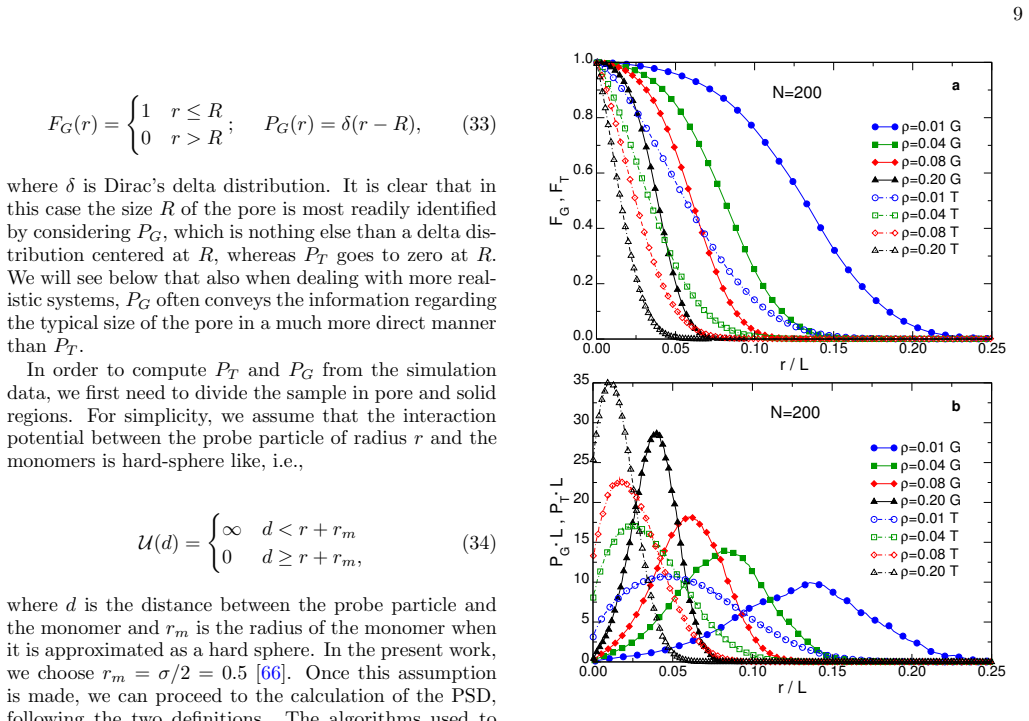
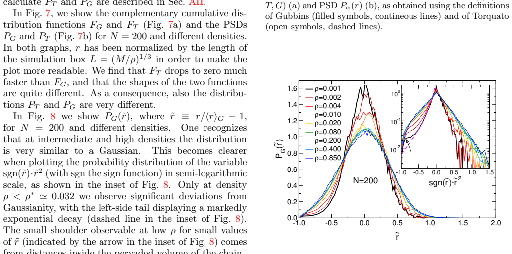
The load-bearing object is the pore size distribution (PSD), computed by two definitions. Torquato's PSD, $P_T(r)$, is the probability density for a random solvent point to lie at distance $r$ from the nearest point on the monomer surface; it is obtained from the fraction of pore volume accessible to the center of a hard probe sphere of radius $r$. Gubbins's PSD, $P_G(r)$, instead assigns to $r$ the volume coverable by spheres of radius $r$ or smaller (the Connolly/reentrant surface), so its mean gives the pore size directly—for an isolated spherical pore $\langle r\rangle_G$ equals the pore radius while $\langle r\rangle_T=R/4$. The argument is carried by the analytic PSD of overlapping spheres, whose mean yields the parameter-free formula Eq. (46); the Puiseux asymptotics of the exponential integral convert this formula into the scaling powers $\chi^{-\nu+1/3}$ and $\chi^{-\nu}$.

What would settle it

Compute the two pore-size distributions at a density just below the concentrated-regime onset, $\rho\approx 0.3$, using two monomer radii, e.g. $r_m=0.4\sigma$ and $r_m=0.6\sigma$. If the resulting means $\langle r\rangle_T$ or $\langle r\rangle_G$ shift by more than the scatter that scaling theory permits, or if $\langle r\rangle_G/\langle r\rangle_T$ departs significantly from $\approx 2$, then the claimed identification of the mesh size with a pore-size mean depends too strongly on the hard-sphere monomer model to be the geometric mesh size.

Watch

Extended reading notes

Core claim

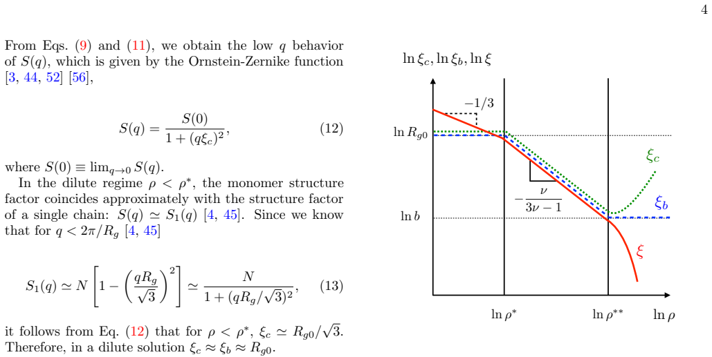
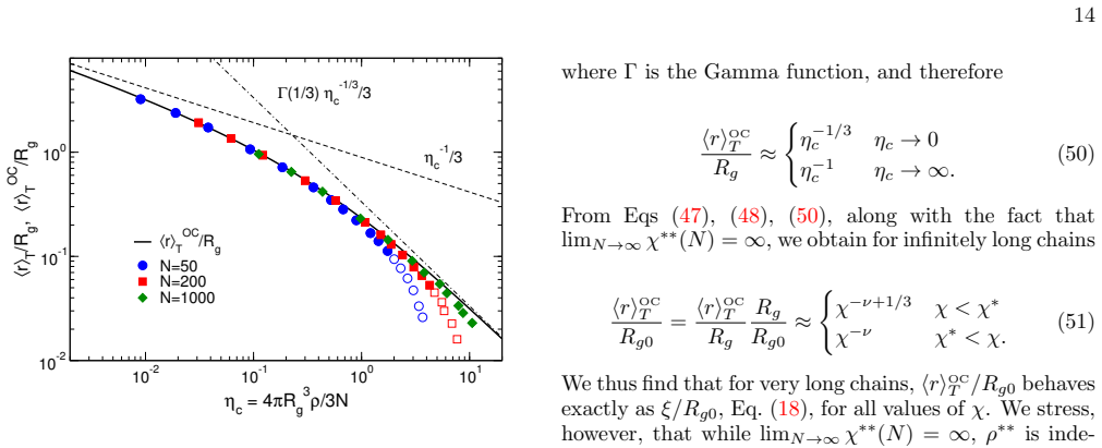
The central claim is that the geometrical mesh size $\xi$ of a polymer solution equals the mean pore size defined by either of the two standard pore-size distributions. Torquato's mean $\langle r\rangle_T$ (distance from a random solvent point to the nearest monomer surface) and Gubbins's mean $\langle r\rangle_G$ (radius of the largest sphere coverable at that point) both collapse onto the scaling prediction $\xi/R_{g0}\propto \chi^{-\nu}$ in the semidilute regime and onto the dilute-limit behavior $\chi^{-\nu+1/3}$, while the density-fluctuation correlation length $\xi_c$ follows this only in the semidilute regime and rises again at high density. The identification is supported by a model polymer gel with known mesh size, where Gubbins's distribution peaks at the true mesh size. The paper further claims that the parameter-free overlapping-chains expression $\langle r\rangle_T^{\mathrm{OC}}=(R_g/3)e^{\eta_c}E_{2/3}(\eta_c)$, with $\eta_c=4\pi R_g^3\rho/(3N)$, reproduces the simulated $\langle r\rangle_T$ in the semidilute regime and asymptotically yields the scaling law for long chains.

Load-bearing premise

The entire pore geometry is built by treating each monomer as a hard sphere of radius $\sigma/2$; whenever the average pore size approaches that monomer radius, the computed means—and hence the identification $\langle r\rangle = \xi$—depend on this modeling choice.

Editorial extensions

If this is right

The mesh size becomes a directly measurable geometric quantity at any density, with no unknown multiplicative prefactor and no dependence on an assumed overlap concentration.
The full distribution of mesh sizes, not just its mean, is accessible; this enables direct study of how spatial heterogeneity of the mesh affects tracer-particle diffusion.
In semidilute solutions, $\langle r\rangle_T$ (and hence, up to the factor $\approx 2$, $\langle r\rangle_G$) can be estimated without simulation or scattering by inserting the radius of gyration and density into Eq. (46).
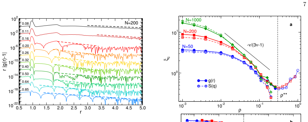
Using $\xi_c$ as a proxy for the mesh size is ruled out except in the semidilute regime, since $\xi_c$ increases with density in concentrated solutions while pore sizes decrease.
The PSD method extends to other polymer topologies and to networks and gels, where the mesh-size distribution is currently hard to access.

Reading between the lines

Editorial extensions of the paper, not claims the author makes directly.

Because Gubbins's mean gives the true pore radius in idealized pores, $\langle r\rangle_G$ is arguably the better proxy for the particle radius separating free from obstructed diffusion; the systematic factor $\langle r\rangle_G/\langle r\rangle_T\approx 2$ should be checked against tracer-diffusion measurements in the same systems.
The overlapping-chains formula implies that the mean pore size is controlled mainly by the chain-level packing variable $R_g^3\rho/N$; in real systems this could let one map measured radii of gyration and concentrations directly onto mesh sizes without any scattering-derived correlation length.
A direct numerical test of the proposed identification would be to compare $\langle r\rangle_G$ with the tracer radius at which the diffusivity crossover occurs in the same simulated solutions; the paper does not perform this comparison.

Share X Bluesky LinkedIn Reddit HN

Signed reviews

No signed human review yet.

Editorial analysis

A structured set of objections, weighed in public.

Desk editor's note, referee report, and a circularity audit.

Desk Editor's Note

read the letter

First thing to know: this paper gives you a practical way to measure mesh size distributions in polymer simulations, not just an average. Second: the quantitative identification of the mean pore size with xi is weaker than the abstract claims, but that doesn't sink the method.

The genuinely new piece is the application of two standard porous-media pore size distributions (Torquato, Gubbins) to polymer solutions, and the overlapping-chains (OC) estimator, Eq. (46), which reproduces _T from Rg and density with no fit parameters. I checked the logic: it uses the analytical Torquato PSD for overlapping spheres and plugs in Rg and chain density. That it works across the semidilute range is a real result. The gel test in Fig. 12 is also a good idea—a system with a known mesh—and it supports the earlier conclusion that Gubbins's PG is the more interpretable distribution. The simulations are standard Kremer-Grest, with proper equilibration checks and several chain lengths; the scaling collapse in Fig. 10 is convincing.

Now the soft spots. The paper's abstract says xi can be identified with either _T or _G, but these two differ by a factor near 2 (Fig. 11b), so at most one can equal xi. The scaling comparison in Fig. 10 fixes only the exponent; any length with the same rho-dependence collapses onto that line. The absolute values also depend on the hard-sphere monomer radius r_m = sigma/2, and near rho** the pores are not much larger than r_m, so the shift is not negligible. The paper does flag this in footnote 66, but the abstract overstates. There are also no error bars on the reported values, and the xi_c fits in the intermediate density range are made with a functional form the authors say is not justified—they are honest about it, but it is a weak point. None of this kills the method; it does mean the quantitative claim should be softened to "both estimators have the same scaling as xi, and PG gives the better absolute estimate," with the gel simulation as the real benchmark.

Who is it for: anyone simulating or interpreting diffusion of nanoparticles or proteins in polymer solutions, and anyone who needs a mesh size distribution rather than a single correlation length. The citation pattern looks appropriate. It deserves a serious referee; I would send it out with a request for error bars and a careful rewrite of the identification claim.

Referee Report

4 major / 5 minor

Summary. The paper uses molecular dynamics simulations of coarse-grained Kremer-Grest polymer chains (N = 50, 200, 1000; monomer densities from 0.001 to 1.0) to characterize the geometrical mesh size ξ of polymer solutions. It measures the monomer density fluctuation correlation length ξ_c from both the static structure factor and the radial distribution function, and computes pore size distributions (PSDs) using the definitions of Torquato and of Gubbins. The authors report that the mean pore sizes ⟨r⟩_T and ⟨r⟩_G both follow the scaling form predicted for ξ in the semidilute regime, and argue that ξ can be identified with either quantity. They also introduce a parameter-free 'overlapping chains' (OC) model, in which the polymer solution is mapped onto overlapping spheres with radius R_g and density ρ/N, and show that the resulting analytical mean ⟨r⟩_T^{OC} reproduces ⟨r⟩_T accurately for ρ < ρ**. A model cubic polymer gel is used as an independent test to argue that Gubbins's PSD is the more direct indicator of the true pore size.

Significance. If the quantitative identification ⟨r⟩ = ξ holds, the paper would provide a direct, distribution-level route to the mesh size, which is more informative than scaling estimates or correlation-length measurements and is relevant for models of nanoparticle diffusion in polymer solutions. The simulation work is careful and standard, and the paper is strong on several counts: it compares two PSD definitions on the same systems, validates Gubbins's PSD against a model gel with independently known mesh size, and derives an elegant parameter-free approximation for ⟨r⟩_T from R_g and ρ. The scaling-exponent agreement in Figs. 10 and 11 is convincing. However, the quantitative identification of both ⟨r⟩_T and ⟨r⟩_G with the same ξ is not established: the two means differ by a factor near 2, the absolute values depend on the arbitrary monomer radius r_m, and the scaling comparison fixes only an exponent with an approximate prefactor.

major comments (4)

[IV C, Figs. 10 and 11] The central claim that ξ can be identified with either ⟨r⟩_T or ⟨r⟩_G is not supported by the evidence presented. The comparison in Fig. 10 tests essentially the semidilute exponent: Eq. (19) carries an unknown O(1) prefactor and uses the approximate overlap density ρ* from Eq. (20), so any length with the same χ-dependence would collapse onto the same line. Fig. 11b shows ⟨r⟩_G/⟨r⟩_T ≈ 2, so at most one of the two means can equal the same numerical ξ. The model-gel test in Fig. 12 independently favors PG rather than PT. The conclusion should therefore be restricted to proportionality (⟨r⟩_T ≈ c_T ξ, ⟨r⟩_G ≈ c_G ξ with c_G/c_T ≈ 2), unless a calibration against an independently known mesh size is supplied.
[IV B, Eq. (34) and footnote [66]] The absolute values of ⟨r⟩_T and ⟨r⟩_G depend on the arbitrary hard-sphere monomer radius r_m = σ/2 used to define the pore-solid interface. The authors acknowledge this in footnote [66], but they do not quantify the sensitivity. Near the operational concentrated-regime onset ρ** = 0.3 the mean pore sizes become comparable to the monomer size (for N = 50, R_g0 ≈ 4.8, so scaling values of ⟨r⟩ are of order unity), and a change of r_m by 0.1σ would shift ⟨r⟩ by a non-negligible fraction. Since the literal identification ⟨r⟩ = ξ is central to the paper, a sensitivity study over r_m is required, at least for the densities where ⟨r⟩ ≈ σ.
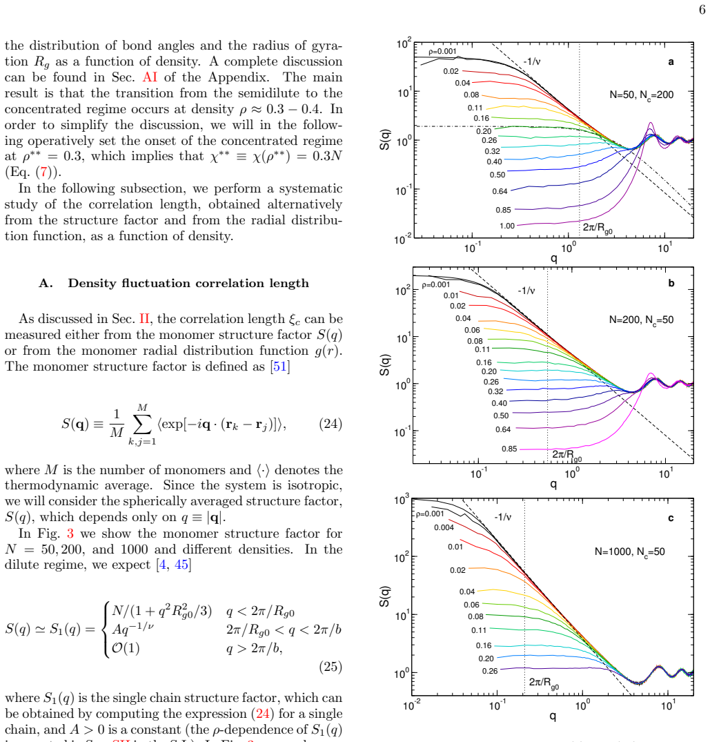
[IV A, Fig. 4] The correlation-length data in Fig. 5 are obtained from fits that the authors themselves describe as not satisfactory in the intermediate density range. In Sec. IV A they state that for densities 0.11 < ρ < 0.64 neither the low-density form Eq. (9) nor the high-density form Eq. (10) gives a really satisfactory description, and that they nevertheless fit with an exponential 'to have at least an estimate'. These ξ_c values are then used in Fig. 10 in comparisons that support the paper's negative conclusions about ξ = ξ_c outside the semidilute regime. The paper should either restrict the ξ_c analysis to the ranges where the functional forms are justified or report fit quality measures that allow the reader to judge the uncertainty.
[IV D, Eqs. (46)-(51), Fig. 17] The OC model is genuinely parameter-free, but the agreement shown in Fig. 17 does not independently certify that ⟨r⟩_T equals ξ. Equation (51) demonstrates that, for long chains, the OC expression reproduces exactly the scaling form of ξ in Eq. (18), because the inputs R_g and η_c are themselves chosen from the same scaling theory. The agreement is therefore partly a consistency check of the scaling ansatz rather than an external validation of the absolute pore size. The text should be revised to present the OC result as a practical estimator of ⟨r⟩_T, not as evidence for the literal identification ⟨r⟩_T = ξ.

minor comments (5)

[Fig. 13 caption] The caption contains a typo: 'Torquato's PDS' should read 'Torquato's PSD'.
[Fig. 7 caption] The caption reads 'contineous lines'; this should be 'continuous lines'.
[Figs. 5, 10, 11, 17] No statistical uncertainties are reported for ⟨r⟩_T, ⟨r⟩_G, or ξ_c. Given that the paper makes quantitative claims about 'high accuracy', error bars or at least a statement of the statistical error from block averaging should be added.
[Fig. 11b] The logarithmic fit line is quoted as 2.18 + 0.0458 ln(χ), but the fit range, the uncertainty of the coefficients, and the goodness of fit are not given. This should be specified.
[II B, Eq. (12)] The derivation of the Ornstein-Zernike form from Eq. (11) is only sketched in footnote [56]; a brief sentence in the main text would make the step clearer.

Circularity Check

1 steps flagged · score 4.0 of 10

The identification ⟨r⟩=ξ is partially definitional because the paper stipulates ξ to be the average pore size; the PSD and OC-model analyses are otherwise self-contained.

self definitional [Sec. I (definition of ξ) and Sec. IV C / Sec. V (identification of ⟨r⟩ with ξ), Eqs. (36) and surrounding text]
"we will in the present work adopt this intuitive concept of ξ as the average pore size of the polymer solution. ... We propose a method to directly probe the geometrical mesh size ξ, which we identify with the average size of the pores of the polymer solution. ... We find that in both cases, the average of the PSD, ⟨r⟩, follows the expected scaling behavior for ξ with high accuracy, validating the hypothesis that ⟨r⟩ can be identified with the geometrical mesh size."

The paper defines ξ as the average pore size in Sec. I, then defines ⟨r⟩_α as the mean pore radius (Eq. (36)), and finally concludes that ⟨r⟩ can be identified with ξ. Given the stipulated definition, that identification is true by construction and requires no empirical test. The scaling comparison in Fig. 10 and Eq. (18) is a consistency check, not an independent derivation of the equality. The ambiguity is visible in the paper's own finding that ⟨r⟩_G and ⟨r⟩_T differ by a factor close to 2, so the definition alone cannot decide which mean is ξ; the paper must invoke the spherical-pore example and the model gel to select Gubbins's PSD. The PSD computation itself is not circular, but the headline identification is partly a definitional reduction.

full rationale

The paper's derivation chain is mostly self-contained: the pore size distributions are computed directly from simulated monomer coordinates, the OC model of Eq. (46) uses only measured R_g and density as inputs rather than parameters fitted to PSD, and the model-gel test in Fig. 12 provides an independent system with a known mesh size. There is no load-bearing self-citation or imported uniqueness theorem. The only significant circular component is the definitional identification of ξ with average pore size, which makes the final statement that ⟨r⟩ can be identified with ξ true by construction rather than by empirical derivation. Because this is one of the paper's central claims but is accompanied by a substantial, independently meaningful PSD analysis, a moderate partial-circularity score is appropriate. The absolute-scale ambiguity from the monomer radius r_m and the factor-of-two difference between ⟨r⟩_G and ⟨r⟩_T are correctness/underdetermination concerns, not additional circularity.

Assumptions & free parameters 3 free parameters · 3 assumptions · 0 invented entities

The central identification ⟨r⟩ = ξ rests on the scaling comparison and on the hard-sphere probe approximation. The only user-chosen parameter for the pore space is r_m = σ/2; ρ** is an operational cutoff. The OC model itself is parameter-free given Rg and ρ, but its validation depends on the simulation data and the scaling framework.

free parameters (3)

monomer hard-sphere radius r_m = 0.5 (in units of σ)
Assumed for partitioning the system into pore and solid regions (Eq. (34), Sec. IV B). Different choices shift the PSD, and the paper only argues the effect is small when pore sizes are much larger than |r_m - r_m'|.
concentrated-regime onset ρ** = 0.3
Set operationally from Rg and bond-angle data (Sec. IV). Used to mark the semidilute/concentrated boundary and to exclude points from some scaling comparisons.
HS/OS fit parameters R_HS, R_OS, ρ_HS, ρ_OS = density-dependent values
Fitted to Torquato's PSD in Sec. IV D to test the sphere-mapping hypothesis. These fits are not used in the parameter-free OC model and do not affect the central estimator.

assumptions (3)

domain assumption Flory exponent ν ≈ 0.588 and blob scaling laws describe semidilute polymer solutions in athermal solvent
Used throughout Sec. II and for comparing the PSD means to scaling predictions (Eqs. (3), (4), (14), (17)).
domain assumption Ornstein-Zernike form S(q) = S(0)/(1 + (qξ_c)^2) and exponential decay of g(r) hold for monomer density fluctuations
Used to extract ξ_c from S(q) and g(r) in Secs. II and IV A (Eqs. (9), (10), (12)).
domain assumption Hard-sphere probe potential between monomers and the probe particle defines the pore space
Eq. (34) in Sec. IV B; the pore/solid boundary is determined by r_m = σ/2. This is a modeling choice that affects the PSD.

how reviews work

0 comments

Cite this review

Pith. "Pith review of Characterizing the mesh size of polymer solutions via the pore size distribution." pith.science (2026). https://pith.science/paper/S67MIP4F

@misc{pith2026190801484,
  author       = {Pith},
  title        = {Pith review of: Characterizing the mesh size of polymer solutions via the pore size distribution},
  year         = {2026},
  howpublished = {\url{https://pith.science/paper/S67MIP4F}},
  note         = {Machine review of arXiv:1908.01484}
}

abstract

In order to characterize the geometrical mesh size $\xi$, we simulate a solution of coarse-grained polymers with densities ranging from the dilute to the concentrated regime and for different chain lengths. Conventional ways to estimate $\xi$ rely either on scaling assumptions which give $\xi$ only up to an unknown multiplicative factor, or on measurements of the monomer density fluctuation correlation length $\xi_c$. We determine $\xi_c$ from the monomer structure factor and from the radial distribution function, and find that the identification $\xi=\xi_c$ is not justified outside of the semidilute regime. In order to better characterize $\xi$, we compute the pore size distribution (PSD) following two different definitions, one by Torquato et al. (Ref.1) and one by Gubbins et al. (Ref.2). We show that the mean values of the two distributions, $\langle r \rangle_T$ and $\langle r \rangle_G$, both display the behavior predicted for $\xi$ by scaling theory, and argue that $\xi$ can be identified with either one of these quantities. This identification allows to interpret the PSD as the distribution of mesh sizes, a quantity which conventional methods cannot access. Finally, we show that it is possible to map a polymer solution on a system of hard or overlapping spheres, for which Torquato's PSD can be computed analytically and reproduces accurately the PSD of the solution. We give an expression that allows $\langle r \rangle_T$ to be estimated with great accuracy in the semidilute regime by knowing only the radius of gyration and the density of the polymers.

Figures

Figures reproduced from arXiv: 1908.01484 by the authors.

**Figure 2.** FIG. 2. Expected [PITH_FULL_IMAGE:figures/full_fig_p004_2.png] view at source ↗

**Figure 3.** FIG. 3. Monomer structure factor [PITH_FULL_IMAGE:figures/full_fig_p006_3.png] view at source ↗

Figures from the paper (13 more)

**Figure 4.** Figure 4: FIG. 4. The function [PITH_FULL_IMAGE:figures/full_fig_p007_4.png]

**Figure 5.** Figure 5: FIG. 5. The length [PITH_FULL_IMAGE:figures/full_fig_p007_5.png]

**Figure 6.** Figure 6: FIG. 6. Example of a porous medium with a single star [PITH_FULL_IMAGE:figures/full_fig_p008_6.png]

**Figure 7.** Figure 7: FIG. 7. Complementary cumulative distribution [PITH_FULL_IMAGE:figures/full_fig_p009_7.png]

**Figure 8.** Figure 8: FIG. 8. Gubbins’s PSD, [PITH_FULL_IMAGE:figures/full_fig_p009_8.png]

**Figure 10.** Figure 10: FIG. 10. Comparison between the average pore sizes, the [PITH_FULL_IMAGE:figures/full_fig_p010_10.png]

**Figure 12.** Figure 12: FIG. 12. PSD for a model polymer gel (cubic lattice with [PITH_FULL_IMAGE:figures/full_fig_p011_12.png]

**Figure 13.** Figure 13: FIG. 13. Torquato’s PDS, [PITH_FULL_IMAGE:figures/full_fig_p012_13.png]

**Figure 14.** Figure 14: FIG. 14. Fit parameters as a function of monomer density [PITH_FULL_IMAGE:figures/full_fig_p012_14.png]

**Figure 15.** Figure 15: FIG. 15. Dimensionless densities [PITH_FULL_IMAGE:figures/full_fig_p013_15.png]

**Figure 17.** Figure 17: FIG. 17. Reduced average pore size [PITH_FULL_IMAGE:figures/full_fig_p014_17.png]

**Figure 18.** Figure 18: FIG. 18. Normalized polymer radius of gyration, Eq. ( [PITH_FULL_IMAGE:figures/full_fig_p015_18.png]

**Figure 19.** Figure 19: FIG. 19. Bond-bond correlation function [PITH_FULL_IMAGE:figures/full_fig_p016_19.png]

Discussion (0). Continue with ORCID to comment.

Reference graph

Works this paper leans on

85 extracted references · 71 canonical work pages

[66]

We note that diﬀerent choices of rm will lead to diﬀerent PSDs. However, given two diﬀerent valuesrm andr′ m, we expect the diﬀerence between the PSDs computed using these two values to be relevant only when the average pore size is comparable to, or smaller than, |rm−r′ m|

work page
[1]

A random point r is chosen in the pore phase
[2]

bHKQGOqI2rfN3Abs9TX3EAIXpVc=

The smallest distancermin between r and the center of a monomer is calculated. The distance between r and the nearest pore-solid interface is calculated as r =rmin−σ/2. This procedure is repeated many times, until a large numberN of r values is recorded. In the limit of large N , the normalized histogram of these values is equivalent to PT (r). B. Gubbins...
[3]

De Gennes, Scaling concepts in polymer physics (Cornell University Press, 1979)

P.-G. De Gennes, Scaling concepts in polymer physics (Cornell University Press, 1979)

1979
[4]

Torquato, B

S. Torquato, B. Lu, and J. Rubinstein, Phys. Rev. A 41, 2059 (1990)

1990
[5]

L. D. Gelb and K. Gubbins, Langmuir 15, 305 (1999)

1999
[6]

Zhou, FEBS Lett

H.-X. Zhou, FEBS Lett. 587, 1053 (2013)

work page 2013
[7]

Rubinstein and R

M. Rubinstein and R. H. Colby, Polymer physics (Oxford University Press, 2003)

2003

Show all 85 references

[8]

H.-X. Zhou, G. Rivas, and A. P. Minton, Annu. Rev. Biophys. 37, 375 (2008)

2008
[9]

B. S. Schuster, J. S. Suk, G. F. Woodworth, and J. Hanes, Biomaterials 34, 3439 (2013)

2013
[10]

K. S. Soppimath, T. M. Aminabhavi, A. R. Kulkarni, and W. E. Rudzinski, J. Controlled Release 70, 1 (2001)

2001
[11]

S. K. Lai, D. E. O’Hanlon, S. Harrold, S. T. Man, Y.-Y. Wang, R. Cone, and J. Hanes, Proc. Natl. Acad. Sci. 104, 1482 (2007)

2007
[12]

Johansson, C

L. Johansson, C. Elvingson, and J. E. Loefroth, Macro- molecules 24, 6024 (1991)

1991
[13]

A. G. Ogston, B. Preston, and J. Wells, Proc. R. Soc. Lond. A 333, 297 (1973)

1973
[14]

A. R. Altenberger and M. Tirrell, J. Chem. Phys. 80, 2208 (1984)

1984
[15]

Cukier, Macromolecules 17, 252 (1984)

R. Cukier, Macromolecules 17, 252 (1984)

1984
[16]

G. D. Phillies, G. S. Ullmann, K. Ullmann, and T.-H. Lin, J. Chem. Phys. 82, 5242 (1985)

1985
[17]

G. D. Phillies, Macromolecules 19, 2367 (1986)

1986
[18]

Tuinier and T.-H

R. Tuinier and T.-H. Fan, Soft Matter 4, 254 (2008)

2008
[19]

Odijk, Biophys

T. Odijk, Biophys. J. 79, 2314 (2000)

2000
[20]

T.-H. Fan, J. K. Dhont, and R. Tuinier, Phys. Rev. E 75, 011803 (2007)

2007
[21]

Y. Dong, X. Feng, N. Zhao, and Z. Hou, J. Chem. Phys. 143, 024903 (2015)

2015
[22]

Egorov, J

S. Egorov, J. Chem. Phys. 134, 084903 (2011)

2011
[23]

Yamamoto and K

U. Yamamoto and K. S. Schweizer, J. Chem. Phys. 135, 224902 (2011)

2011
[24]

Kohli and A

I. Kohli and A. Mukhopadhyay, Macromolecules45, 6143 (2012)

2012
[25]

Masaro and X

L. Masaro and X. Zhu, Prog. Polym. Sci. 24, 731 (1999)

1999
[26]

L.-H. Cai, S. Panyukov, and M. Rubinstein, Macro- molecules 44, 7853 (2011)

2011
[27]

R. Chen, R. Poling-Skutvik, A. Nikoubashman, M. P. Howard, J. C. Conrad, and J. C. Palmer, Macro- molecules 51, 1865 (2018)

2018
[28]

Babaye Khorasani, R

F. Babaye Khorasani, R. Poling-Skutvik, R. Krish- namoorti, and J. C. Conrad, Macromolecules 47, 5328 (2014)

2014
[29]

Poling-Skutvik, R

R. Poling-Skutvik, R. Krishnamoorti, and J. C. Conrad, ACS Macro Lett. 4, 1169 (2015)

2015
[30]

Z. E. Dell and K. S. Schweizer, Macromolecules 47, 405 (2013). 20

2013
[31]

R. Chen, R. Poling-Skutvik, M. P. Howard, A. Nikoubashman, S. A. Egorov, J. C. Conrad, and J. C. Palmer, Soft Matter (2019)

2019
[32]

S. R. Lustig and N. A. Peppas, J. Appl. Polym. Sci. 36, 735 (1988)

1988
[33]

Parrish, M

E. Parrish, M. A. Caporizzo, and R. J. Composto, J. Chem. Phys. 146, 203318 (2017)

2017
[34]

S. Rose, A. Marcellan, D. Hourdet, C. Creton, and T. Narita, Macromolecules 46, 4567 (2013)

2013
[35]

L.-H. Cai, S. Panyukov, and M. Rubinstein, Macro- molecules 48, 847 (2015)

2015
[36]

Scheidegger, The physics of ﬂow through porous media (Macmillan, 1957)

A. Scheidegger, The physics of ﬂow through porous media (Macmillan, 1957)

1957
[37]

Parrish, S

E. Parrish, S. C. Seeger, and R. J. Composto, Macro- molecules 51, 3597 (2018)

2018
[38]

Koshy, T

R. Koshy, T. Desai, P. Keblinski, J. Hooper, and K. Schweizer, J. Chem. Phys. 119, 7599 (2003)

2003
[39]

Torquato, Phys

S. Torquato, Phys. Rev. E 51, 3170 (1995)

1995
[40]

Prager, Chem

S. Prager, Chem. Eng. Sci. 18, 227 (1963)

1963
[41]

Torquato and M

S. Torquato and M. Avellaneda, J. Chem. Phys. 95, 6477 (1991)

1991
[42]

Pikunic, C

J. Pikunic, C. Clinard, N. Cohaut, K. E. Gubbins, J.-M. Guet, R. J.-M. Pellenq, I. Rannou, and J.-N. Rouzaud, Langmuir 19, 8565 (2003)

2003
[43]

Torquato, Random heterogeneous materials: mi- crostructure and macroscopic properties (Springer Sci- ence & Business Media, 2013)

S. Torquato, Random heterogeneous materials: mi- crostructure and macroscopic properties (Springer Sci- ence & Business Media, 2013)

2013
[44]

K. T. Thomson and K. E. Gubbins, Langmuir 16, 5761 (2000)

2000
[45]

Teraoka, Polymer solutions: an introduction to physical properties (John Wiley & Sons, 2002)

I. Teraoka, Polymer solutions: an introduction to physical properties (John Wiley & Sons, 2002)

2002
[46]

Bhattacharya and K

S. Bhattacharya and K. E. Gubbins, Langmuir 22, 7726 (2006)

2006
[47]

Doi and S

M. Doi and S. F. Edwards, The theory of polymer dy- namics (Oxford University Press, 1988)

1988
[48]

W. Paul, K. Binder, D. W. Heermann, and K. Kremer, J. Phys. II 1, 37 (1991)

1991
[49]

Clisby, Phys

N. Clisby, Phys. Rev. Lett. 104, 055702 (2010)

2010
[50]

We are assuming here that b≈ σ, with σ the monomer size, and that the solvent is athermal, so that the size of the thermal blob is approximately equal to b
[51]

Hansen and I

J.-P. Hansen and I. R. McDonald, Theory of simple liq- uids (Elsevier, 1990)

1990
[52]

Gerroﬀ, A

I. Gerroﬀ, A. Milchev, K. Binder, and W. Paul, J. Chem. Phys. 98, 6526 (1993)

1993
[53]

We choose to use χ and not ρ/ρ∗ as a scaling variable since ρ∗ is not a sharply deﬁned quantity
[54]

Evans, R

R. Evans, R. Leote de Carvalho, J. Henderson, and D. Hoyle, J. Chem. Phys. 100, 591 (1994)

1994
[55]

M. E. Fisher, J. Math. Phys. 5, 944 (1964)

1964
[56]

Verlet, Phys

L. Verlet, Phys. Rev. 165, 201 (1968)

1968
[57]

Kremer and G

K. Kremer and G. S. Grest, J. Chem. Phys. 92, 5057 (1990)

1990
[58]

Evans, J

R. Evans, J. Henderson, D. Hoyle, A. Parry, and Z. Sabeur, Mol. Phys. 80, 755 (1993)

1993
[59]

(12) follows formally from Eq

To be more precise, Eq. (12) follows formally from Eq. (11) if g(r) = 1 + Ae−r/ξc/r− δ(r)/ρ. The pres- ence of the delta distribution is however only an artifact stemming from the fact that we are connecting the large r behavior of g(r) with the small q behavior of S(q). In an...
[60]

Schneider and E

T. Schneider and E. Stoll, Phys. Rev. B 17, 1302 (1978)

1978
[61]

J. D. Weeks, D. Chandler, and H. C. Andersen, J. Chem. Phys. 54, 5237 (1971)

1971
[62]

Plimpton, J

S. Plimpton, J. Comput. Phys. 117, 1 (1995)

1995
[63]

In the def- inition of Do et al

Other deﬁnitions of the PSD are possible. In the def- inition of Do et al. (J. Colloid Interface Sci. 328, 110 (2008)), for example, the void-solid interface is the boundary of the region D such that if the center of the probe particle is inD, the solid-probe interaction energ...

2008
[64]

R. Auhl, R. Everaers, G. S. Grest, K. Kremer, and S. J. Plimpton, J. Chem. Phys. 119, 12718 (2003)

2003
[65]

M. L. Connolly, J. Appl. Crystallogr. 16, 548 (1983)

1983
[67]

Lee and F

B. Lee and F. M. Richards, J. Mol. Bio. 55, 379 (1971)

1971
[68]

F. M. Richards, Annu. Rev. Biophys. Bio. 6, 151 (1977)

1977
[69]

Rintoul, S

M. Rintoul, S. Torquato, C. Yeong, D. Keane, S. Er- ramilli, Y. Jun, D. Dabbs, and I. Aksay, Phys. Rev. E 54, 2663 (1996)

1996
[70]

Abramowitz and I

M. Abramowitz and I. A. Stegun,Handbook of mathemat- ical functions: with formulas, graphs, and mathematical tables (Courier Corporation, 1965)

1965
[71]

J. H. Davenport, Y. Siret, , and E. Tournier, Computer Algebra: Systems and Algorithms for Algebraic Compu- tation (2nd ed.) (Academic press, 1993)

1993
[72]

Wittmer, H

J. Wittmer, H. Meyer, J. Baschnagel, A. Johner, S. Obukhov, L. Mattioni, M. M¨ uller, and A. N. Semenov, Physical review letters 93, 147801 (2004)

2004
[73]

Tsuji, X

Y. Tsuji, X. Li, and M. Shibayama, Gels 4, 50 (2018)

2018
[74]

E. R. Duering, K. Kremer, and G. S. Grest, J. Chem. Phys. 101, 8169 (1994)

1994
[75]

Hsu and K

H.-P. Hsu and K. Kremer, J. Chem. Phys. 144, 154907 (2016)

2016
[76]

Sch¨ afer and K

L. Sch¨ afer and K. Elsner, The European Physical Journal E 13, 225 (2004)

2004
[77]

H.-P. Hsu, W. Paul, and K. Binder, Macromolecules 43, 3094 (2010)

2010
[78]

T. H. Rowan, Functional Stability Analysis of Numeri- cal Algorithms, Ph.D. thesis, Department of Computer Sciences, University of Texas at Austin (1990)

1990
[79]

W. H. Press, S. A. Teukolsky, W. T. Vetterling, and B. P. Flannery, Numerical recipes 3rd edition: The art of scientiﬁc computing (Cambridge university press, 2007)

2007
[80]

The nlopt nonlinear-optimization pack- age,

S. G. Johnson, “The nlopt nonlinear-optimization pack- age,” http://github.com/stevengj/nlopt
[81]

L. J. Fetters, D. J. Lohse, S. T. Milner, and W. W. Graessley, Macromolecules 32, 6847 (1999)

1999
[82]

R. S. Hoy, K. Foteinopoulou, and M. Kr¨ oger, Phys. Rev. E 80, 31803 (2009)

2009
[83]

Fetters, D

L. Fetters, D. Lohse, D. Richter, T. Witten, and A. Zirkel, Macromolecules 27, 4639 (1994)

1994
[85]

Kr¨ oger and S

M. Kr¨ oger and S. Hess, Phys. Rev. Lett.85, 1128 (2000)

2000
[200]

(null)">(null)</latexit><latexit sha1_base64=

The dashed lines are exponential ﬁts. ent chain lengths, we note that for densities ρ >0.11≃ ρ∗(N = 50) (see Eq. (20)), S(q) becomes independent of N (see Fig. S3 in the S.I.). This is in agreement with the prediction that in the semidilute and concentrated regimes, ρ>ρ ∗, the...

Pith tools

Reviewed August 14, 2026 · model on record in the stance chip above.

[1] [66]

We note that diﬀerent choices of rm will lead to diﬀerent PSDs. However, given two diﬀerent valuesrm andr′ m, we expect the diﬀerence between the PSDs computed using these two values to be relevant only when the average pore size is comparable to, or smaller than, |rm−r′ m|

work page

[2] [1]

A random point r is chosen in the pore phase

[3] [2]

bHKQGOqI2rfN3Abs9TX3EAIXpVc=

The smallest distancermin between r and the center of a monomer is calculated. The distance between r and the nearest pore-solid interface is calculated as r =rmin−σ/2. This procedure is repeated many times, until a large numberN of r values is recorded. In the limit of large N , the normalized histogram of these values is equivalent to PT (r). B. Gubbins...

[4] [3]

De Gennes, Scaling concepts in polymer physics (Cornell University Press, 1979)

P.-G. De Gennes, Scaling concepts in polymer physics (Cornell University Press, 1979)

1979

[5] [4]

Torquato, B

S. Torquato, B. Lu, and J. Rubinstein, Phys. Rev. A 41, 2059 (1990)

1990

[6] [5]

L. D. Gelb and K. Gubbins, Langmuir 15, 305 (1999)

1999

[7] [6]

Zhou, FEBS Lett

H.-X. Zhou, FEBS Lett. 587, 1053 (2013)

work page 2013

[8] [7]

Rubinstein and R

M. Rubinstein and R. H. Colby, Polymer physics (Oxford University Press, 2003)

2003