REVIEW 3 major objections 6 minor 23 references
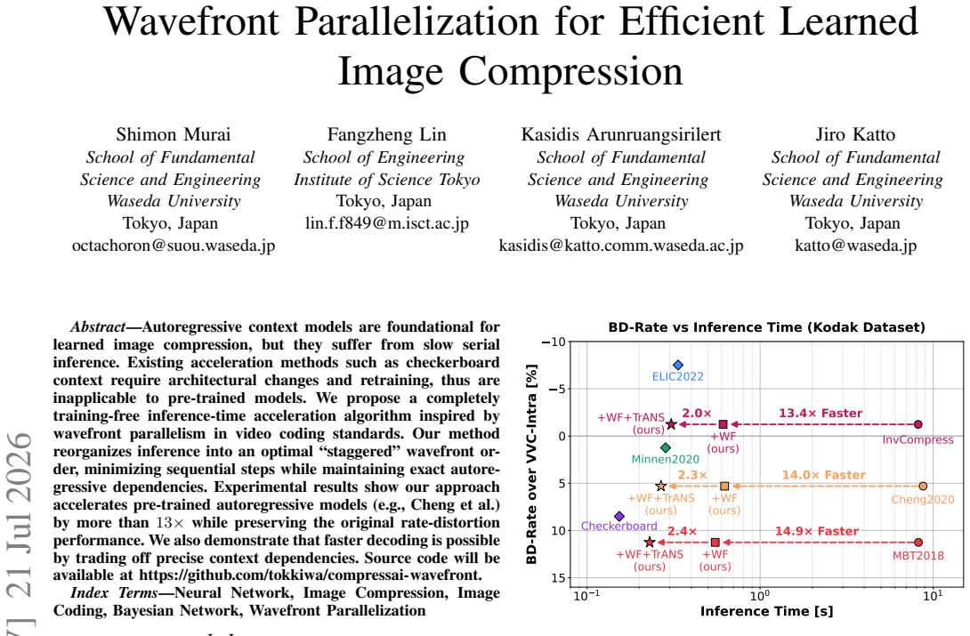
A wavefront scheduling trick accelerates learned image compression by over 13x without retraining.
Reviewed by Pith at T0; open to challenge. T0 means a machine referee read the full paper against a public rubric. the ladder, T0–T4 →
T0 review · deepseek-v4-flash
2026-08-01 13:28 UTC pith:SSPBWA2L
load-bearing objection Scheduling proof is solid and the training-free wavefront acceleration is a real contribution, but the speedup numbers deserve scrutiny before you trust the headline factor. the 3 major comments →
Wavefront Parallelization for Efficient Learned Image Compression
The pith
A machine-rendered reading of the paper's core claim, the machinery that carries it, and where it could break.
Core claim
The central discovery is that the dependency graph of a raster-scan causal masked convolution is sparse enough to admit an optimal parallel schedule: the 'staggered wavefront' order tau(i,j) = (R+1)i + j. For a (2R+1)x(2R+1) kernel, the upper-right neighbor at offset (1,-2) is the critical constraint, forcing shear factor lambda > 2; the minimal integer lambda = 3 for a 5x5 kernel. The paper proves, via Lamport's hyperplane method and a critical-path argument, that this schedule both respects every causal edge and achieves the minimum possible makespan. Since the schedule only reorders independent computations, a pre-trained model can be run in this order with no weight changes, preserving r
What carries the argument
The central object is the staggered wavefront schedule with shear factor lambda = R+1, defined by tau(i,j) = (R+1)i + j. It is derived from Lamport's hyperplane method, which requires a linear schedule vector pi = (lambda,1) such that pi * d > 0 for every dependence vector d in the mask's dependency set D_R = ({1..R} x {-R..R}) union ({0} x {1..R}). The machinery converts the serial raster-scan dependency graph into parallel batches (wavefronts), each decodable in one batched convolution call.
Load-bearing premise
The wavefront schedule preserves exact autoregressive context only if the pretrained model's causal mask is exactly the assumed dependency set D_R — all pixels in R rows above within horizontal offset R, plus R pixels to the left in the same row — with no extra current-row offsets, non-causal padding, or channel-wise dependencies.
What would settle it
Take a pretrained spatial autoregressive model whose 5x5 masked convolution includes an extra dependence on the pixel at offset (1, -3) (one row up, three columns left, outside the assumed {1..2}x{-2..2} set). Run the wavefront schedule tau = 3i + j and compare the decoded latent tensor to the raster-scan decode: if the wavefront order ever evaluates a pixel before that (1,-3) neighbor is available, the two bitstreams will diverge, and the rate-distortion numbers will change, falsifying the claim that the schedule is universally valid.
If this is right
- Pre-trained spatial autoregressive codecs such as Cheng2020, MBT2018, and InvCompress can be accelerated at inference time by 13–72x depending on image size and entropy-coder optimization, with no retraining and no change in rate-distortion performance.
- The theoretical result extends to any (2R+1)x(2R+1) causal mask, giving a simple formula for the optimal shear factor and thus a direct recipe for parallelizing models with larger receptive fields.
- A single trained model can serve multiple speed settings via the context-approximation mode: grouping N consecutive wavefronts and filling unavailable context with mean-fill increases parallelism at a predictable bitrate cost (e.g., +9.7% BPP for N=2, +27.9% for N=4 on Kodak).
- Wavefront parallelization is orthogonal to entropy-coder optimizations: once the neural network is parallelized, the bottleneck shifts to entropy coding, so combining with a tensorized rANS interface yields the largest gains.
- The method is a drop-in replacement for inference on any pre-trained spatial autoregressive model whose mask matches the assumed dependency set, making it directly deployable without modifying model weights.
Where Pith is reading between the lines
- A testable extension: the same optimal-schedule argument should apply to 2D causal masked convolutions in other domains (e.g., audio or video generation) where the dependency set is strictly local and raster-scan ordered; the shear factor formula would carry over directly.
- When combined with channel-wise autoregressive context (as in some hybrid models), the wavefront schedule could parallelize the spatial part while keeping channel dependencies serial, potentially yielding compound speedups rather than a blocking limitation.
- The context-approximation mode implicitly defines a family of approximate posterior distributions; one could train a model specifically for a target group size N, which would likely recover most of the bitrate loss shown in Table II while retaining the speed benefit.
- The theoretical optimality holds in an infinite-processor model; on real GPUs, the practical speedup depends on wavefront width versus the number of resident threads, so an implementation that further splits wide wavefronts or overlaps them could extract additional gains beyond the reported numbers.
Editorial analysis
A structured set of objections, weighed in public.
Referee Report
Summary. This paper proposes a training-free inference-time acceleration method for spatial autoregressive context models in learned image compression. The method models the causal context as a DAG and uses Lamport's hyperplane method to derive a staggered wavefront schedule τ(i,j)=(R+1)i+j, claimed valid and optimal for (2R+1)×(2R+1) raster-scan causal masked convolutions. The authors implement GPU-friendly batching (selective im2col) and a tensorized rANS interface, and report that pre-trained Cheng2020/MBT2018/InvCompress models achieve 13–72× speedups with unchanged BD-rate. An optional context-approximation mode trades bitrate for additional parallelism.
Significance. If the claims hold, this is a useful systems contribution: it accelerates existing pre-trained spatial-AR codecs without retraining, unlike checkerboard or channel-wise replacements. The theoretical derivation is clean and parameter-free: λ=R+1 is forced by the dependency vector (1,-R), and optimality is proven by a critical-path lower bound. The RD preservation shown in Table I is strong evidence that the schedule is exact for the tested models. The main weaknesses are the unvalidated timing methodology and a few table ambiguities.
major comments (3)
- [§IV.A, Tables I and III] The headline speedup claim rests on single-run timings. The data are physically inconsistent: the RTX 2080 SUPER baseline decode for Cheng2020 in Table III is 5.636 s, faster than the RTX 3080 measurement of 5.937 s in Table I; the same inversion appears for the WF runs (0.372 vs 0.4629 s). This indicates uncontrolled GPU state, driver, or CPU differences. Please report mean±std over at least 10 runs, with GPU clocks fixed and identical software stack, and state the number of runs. Without this, the 13–72× numbers cannot be taken at face value.
- [Tables II and IV, §V.D] The 'Wavefront' speeds in Table II (Enc/Dec 21.87/42.71) and Table IV (0.148 s) match the 'WF+TrANS' rows in Table I, not 'WF' alone (0.1606/0.4629). Because Tensorized rANS is a separate engineering contribution, the tables as printed overstate the contribution of the wavefront schedule itself. Please label the exact configuration in every speed column (e.g., 'WF+TrANS') and add a row for WF alone in Table II/IV.
- [Appendix A, Definition 1 / Theorem 1; §III.B] The theorem is stated for the exact dependency set D_R. The text in Section III.B generalizes this to 'any (2R+1)×(2R+1) masked convolution' without proving that every such model has D_R as its dependency set. Practical models may use stacked convolutions, padding, or different mask masks. Please either (i) inspect and report the actual masks of the three evaluated models and confirm they induce D_R, or (ii) restate the theorem as conditional on the model matching D_R. This is important because if a model's effective dependency set is smaller, the schedule may be valid but non-optimal, and the 'optimal' claim would not apply.
minor comments (6)
- [§III.B] 'More generality' should be 'More generally'; typo.
- [§V.E] 'our wavefront methods is applicable' should be 'our wavefront method is applicable'.
- [Table II] Add a footnote stating which implementation (selective im2col, tensorized rANS) each speed row uses; the current row 'Wavefront' appears to include TrANS.
- [Figure 2] Define R for the λ=2 and λ=3 examples; readers may infer that λ=2 is valid for a 5×5 mask, which it is not.
- [Table IV] Specify whether 'Speed (s)' is decode-only or end-to-end; the table header is ambiguous compared to Table I.
- [Reproducibility] The paper says 'source code will be available' but no link to a working repository is provided at review time; please ensure open-source release before publication.
Circularity Check
No significant circularity: the wavefront schedule and optimality proof are derived from the stated dependency set, and pretrained models serve only as external benchmarks.
full rationale
The paper's central derivation is self-contained. The shear factor λ = R+1 is not fitted; it is forced by the validity condition π·d > 0 for all d in the explicit dependency set D_R (Appendix A, Definition 1), with the binding constraint (1,−R) giving λ ≥ R+1. The optimality argument is a matching critical-path lower bound, not a restatement of the schedule: Lemma (2) constructs a directed path of length λI+J−λ using edges (0,1) and (1,−R), and the upper bound is the number of level sets of τ(i,j)=λi+j. Lamport's hyperplane method [10] is an external scheduling-theoretic theorem, and the paper's own equations carry the reduction; no parameter is fitted to the timing or RD results. The pretrained models cited, including Cheng2020 with a co-author overlap, are used only as input benchmarks whose weights are unchanged; the measured RD preservation (BD-rate unchanged at 5.31%, etc.) is an experimental check, not an assumption fed into the proof. The optional context-approximation mode explicitly approximates unavailable context and reports resulting bitrate increases, so it does not masquerade as an exact prediction. The inconsistent GPU timing across settings in Tables I and III is a legitimate correctness/reproducibility concern, but it is not a circularity issue: the speedup numbers do not enter the derivation of the schedule or the optimality theorem. No circular step satisfying the quoted-evidence requirement was found.
Axiom & Free-Parameter Ledger
free parameters (2)
- Group size N (context approximation mode)
- Unknown-context fill constant =
0
axioms (5)
- standard math Lamport's hyperplane method gives valid linear schedules for uniform DAGs when pi dot d > 0 for all dependence vectors d.
- standard math Critical path length lower-bounds makespan in unit-time, infinite-processor scheduling.
- domain assumption Pretrained spatial autoregressive context models have exactly the dependency set D_R: R rows above within horizontal offset R, plus R pixels to the left in the same row.
- domain assumption Batched GPU execution and tensorized rANS preserve the same probability model up to negligible floating-point differences.
- domain assumption In context approximation mode, encoder and decoder compute identical deterministic mean-fill/zero-fill provisional values, keeping entropy coding synchronized.
Cite this review
Pith. "Pith review of Wavefront Parallelization for Efficient Learned Image Compression." pith.science (2026). https://pith.science/paper/SSPBWA2L
@misc{pith2026260719082,
  author       = {Pith},
  title        = {Pith review of: Wavefront Parallelization for Efficient Learned Image Compression},
  year         = {2026},
  howpublished = {\url{https://pith.science/paper/SSPBWA2L}},
  note         = {Machine review of arXiv:2607.19082}
}
read the original abstract
Autoregressive context models are foundational for learned image compression,but they suffer from slow serial inference. Existing acceleration methods such as checkerboard context require architectural changes and retraining, thus are inapplicable to pre-trained models. We propose a completely training-free inference-time acceleration algorithm inspired by wavefront parallelism in video coding standards. Our method reorganizes inference into an optimal ``staggered'' wavefront order, minimizing sequential steps while maintaining exact autoregressive dependencies. Experimental results show our approach accelerates pre-trained autoregressive models (e.g., Cheng et al.) by more than $13\times$ while preserving the original rate-distortion performance. We also demonstrate that faster decoding is possible by trading off precise context dependencies. Source code will be available at https://github.com/tokkiwa/compressai-wavefront.
Figures


Reference graph
Works this paper leans on
-
[1]
Joint autore- gressive and hierarchical priors for learned image compression,
David Minnen, Johannes Ball ´e, and George D Toderici, “Joint autore- gressive and hierarchical priors for learned image compression,” in Advances in Neural Information Processing Systems (NeurIPS), 2018, vol. 31
2018
-
[2]
Learned Image Compression With Discretized Gaussian Mixture Like- lihoods and Attention Modules,
Zhengxue Cheng, Heming Sun, Masaru Takeuchi, and Jiro Katto, “Learned Image Compression With Discretized Gaussian Mixture Like- lihoods and Attention Modules,” inIEEE/CVF Conference on Computer Vision and Pattern Recognition, June 2020
2020
-
[3]
ELIC: Efficient Learned Image Compression With Unevenly Grouped Space-Channel Contextual Adaptive Coding,
Dailan He, Ziming Yang, Weikun Peng, Rui Ma, Hongwei Qin, and Yan Wang, “ELIC: Efficient Learned Image Compression With Unevenly Grouped Space-Channel Contextual Adaptive Coding,” inIEEE/CVF Conference on Computer Vision and Pattern Recognition, 2022, pp. 5718–5727
2022
-
[4]
Checkerboard Context Model for Efficient Learned Image Com- pression,
Dailan He, Yaoyan Zheng, Baocheng Sun, Yan Wang, and Hongwei Qin, “Checkerboard Context Model for Efficient Learned Image Com- pression,” inIEEE/CVF Conference on Computer Vision and Pattern Recognition, 2021, pp. 14766–14775
2021
-
[5]
Channel-Wise Autoregressive Entropy Models for Learned Image Compression,
David Minnen and Saurabh Singh, “Channel-Wise Autoregressive Entropy Models for Learned Image Compression,” inInternational Conference on Image Processing, Oct. 2020, pp. 3339–3343
2020
-
[6]
LVQ-V AE: End-to-end hyperprior-based variational image compression with lattice vector quantization,
Shinobu Kudo, Yukihiro Bandoh, Seishi Takamura, and Masaki Ki- tahara, “LVQ-V AE: End-to-end hyperprior-based variational image compression with lattice vector quantization,” OpenReview, 2023
2023
-
[7]
Approaching rate-distortion limits in neural compression with lattice transform cod- ing,
Eric Lei, Hamed Hassani, and Shirin Saeedi Bidokhti, “Approaching rate-distortion limits in neural compression with lattice transform cod- ing,” inInternational Conference on Learning Representations, 2025
2025
-
[8]
Kodak lossless true color image suite,
“Kodak lossless true color image suite,” https://r0k.us/graphics/kodak/
-
[9]
Enhanced invertible encoding for learned image compression,
Yueqi Xie, Ka Leong Cheng, and Qifeng Chen, “Enhanced invertible encoding for learned image compression,” inProceedings of the 29th ACM International Conference on Multimedia, 2021, p. 162–170
2021
-
[10]
The parallel execution of do loops,
Leslie Lamport, “The parallel execution of do loops,”Communications of the ACM, vol. 17, no. 2, 1974
1974
-
[11]
Auto-encoding variational bayes,
Diederik P Kingma and Max Welling, “Auto-encoding variational bayes,” inInternational Conference on Learning Representations, 2014
2014
-
[12]
End-to-end optimized image compression,
Johannes Ball ´e, Valero Laparra, and Eero P. Simoncelli, “End-to-end optimized image compression,” inInternational Conference on Learning Representations, 2017
2017
-
[13]
Variational image compression with a scale hyperprior,
Johannes Ball ´e, David Minnen, Saurabh Singh, Sung Jin Hwang, and Nick Johnston, “Variational image compression with a scale hyperprior,” inInternational Conference on Learning Representations, 2018
2018
-
[14]
Vivienne Sze, Madhukar Budagavi, and Gary J Sullivan,High efficiency video coding: algorithms and architectures, Springer Publishing Com- pany, 2014
2014
-
[15]
Hevc complexity and implementation analysis,
Frank Bossen, Benjamin Bross, Karsten Suhring, and David Flynn, “Hevc complexity and implementation analysis,”IEEE Transactions on Circuits and Systems for Video Technology, vol. 22, no. 12, 2012
2012
-
[16]
CompressAI: A PyTorch library and evaluation platform for end-to-end compression research,
Jean B ´egaint, Fabien Racap ´e, Simon Feltman, and Akshay Pushparaja, “CompressAI: A PyTorch library and evaluation platform for end-to-end compression research,”arXiv preprint arXiv:2011.03029, 2020
Pith/arXiv arXiv 2011
-
[17]
Calculation of average psnr differences between rd-curves,
Gisle Bjøntegaard, “Calculation of average psnr differences between rd-curves,”ITU-T VCEG-M33, 2001
2001
-
[18]
Jarek Duda, “Asymmetric numeral systems,”arXiv preprint arXiv:1311.2540, 2009
Pith/arXiv arXiv 2009
-
[19]
Testimages: a large-scale archive for testing visual devices and basic image processing algorithms.,
Nicola Asuni, Andrea Giachetti, et al., “Testimages: a large-scale archive for testing visual devices and basic image processing algorithms.,” in Smart Tools and Applications in Graphics(STAG), 2014, pp. 63–70
2014
-
[20]
Work- shop and challenge on learned image compression,
George Toderici, Wenzhe Shi, Radu Timofte, Lucas Theis, Johannes Ball´e, Eirikur Agustsson, Nick Johnston, and Fabian Mentzer, “Work- shop and challenge on learned image compression,” 2020
2020
-
[21]
A cross channel context model for latents in deep image compression,
Changyue Ma, Zhao Wang, Ruling Liao, and Yan Ye, “A cross channel context model for latents in deep image compression,”arXiv preprint arXiv:2103.02884, 2021. APPENDIXA PROOF OF THEVALIDITY ANDOPTIMALITY OF WAVEFRONTPARALLELIZATION In this section, we provide a formal proof of the validity and optimality of the wavefront parallelization strategy in general...
Pith/arXiv arXiv 2021
-
[22]
The staggered wavefront schedule is valid forD R
-
[23]
Proof.(1)Validity.For anyd∈D R, we have π·d= ( p, d= (0, p), p∈ {1,
In the unit-time, infinite-processor model, the staggered wavefront schedule is optimal, i.e., it achieves the mini- mum possible makespan T=λI+J−λ= (R+ 1)I+J−(R+ 1). Proof.(1)Validity.For anyd∈D R, we have π·d= ( p, d= (0, p), p∈ {1, . . . , R}, λr+q, d= (r, q), r∈ {1, . . . , R}, q∈ {−R, . . . , R}. In the first case,π·d=p≥1. In the second case, the min...
discussion (0)
Sign in with ORCID, Apple, or X to comment. Anyone can read and Pith papers without signing in.