Non-Asymptotic Variational Learning for Monotone Nonlinear Multiscale Elliptic Equations: Scale-Robust Primal-Dual Bounds and Strong-Form Statistical Ill-Conditioning

Ronald Katende

REVIEW 2 major objections 3 minor 11 references

For nonlinear multiscale elliptic PDEs, variational and primal–dual learning keep every error constant scale-independent, while strong-form residual classes suffer an intrinsic 1/(ε√N) statistical floor.

Reviewed by Pith at T0; open to challenge. T0 means a machine referee read the full paper against a public rubric. the ladder, T0–T4 →

Challenge this review Re-run · record.json Download PDF Read on arXiv ↗

T0 review · deepseek-v4-flash

2026-08-01 22:32 UTC pith:SWY4F54J

load-bearing objection Worth engaging: the strong-form lower bounds are new and likely correct, but the advertised primal-dual certificate rests on an unproven higher-regularity assumption that should be flagged to any referee. the 2 major comments →

arxiv 2607.15702 v2 pith:SWY4F54J submitted 2026-07-17 math.NA cs.LGcs.NAmath.AP

Non-Asymptotic Variational Learning for Monotone Nonlinear Multiscale Elliptic Equations: Scale-Robust Primal-Dual Bounds and Strong-Form Statistical Ill-Conditioning

Ronald Katende This is my paper

classification math.NA cs.LGcs.NAmath.AP MSC 35B2765N1265N1568T07

keywords multiscale elliptic equationsperiodic homogenizationuniformly monotone nonlinear PDEsvariational physics-informed learningprimal-dual gapRademacher complexitycorrector-enriched trial spacesnon-asymptotic error bounds

verification ladder T0 review T1 audit T2 compute T3 formal T4 reserved

The pith

A machine-rendered reading of the paper's core claim, the machinery that carries it, and where it could break.

This paper develops a non-asymptotic error theory for learning solutions of uniformly monotone nonlinear multiscale elliptic equations, where coefficients oscillate on a small scale ε. It proves that variational energy losses and a new convex primal–dual physics loss produce error bounds whose sampling, stability, and optimization constants are independent of ε, provided the trial classes include a two-scale corrector term. In contrast, it proves that strong-form residual losses have empirical Rademacher complexity growing at least as 1/(ε√N), and squared strong losses at least as 1/(ε²√N), in every spatial dimension and independently of the optimizer. The practical consequence is a formulation-level diagnosis: variational and primal–dual schemes avoid an intrinsic statistical ill-conditioning that strong-form residual learning suffers when the coefficient oscillates. Numerical experiments in d=1,2,3 confirm the predicted ε- and N-scalings and show the primal–dual gap reliably certifies the state error.

Core claim

The paper's central claim is a separation between formulations by scale-robustness. For the variational energy formulation, the state error decomposes into an approximation term, an empirical quadrature term, and a projected-gradient term, with all non-approximation constants uniform in ε; a corrector-enriched two-scale state class closes the approximation term with a bound C(ε + Φ₀² + Φ₁²) in arbitrary dimension. For a new convex primal–dual loss, the population value is a computable upper certificate for the state error, and with an additional flux-corrector regularity assumption, a divergence-compatible two-scale flux class closes the flux approximation, giving a certified state–flux boun

What carries the argument

Two mechanisms carry the argument. The upper bound uses the corrector-enriched two-scale trial class v = U(x) + ε ηε(x) C(x, x/ε), built from the periodic homogenization corrector; its gradient features are ε-uniform because the fast derivative is absorbed by the cutoff and cell derivative. The upper certificate uses the convex primal–dual gap Gε(v,p) = Jε(v) + ∫[F*(x,x/ε,p) + G*(x, f+∇·p)] dx, whose population value bounds the state error from above via Fenchel–Young and equals zero at the exact pair (uε, pε). The lower bound uses a fixed smooth trial state v⋆: the chain rule expresses its strong residual as -(1/ε)H(x/ε, ∇v⋆) plus bounded terms, and the nondegeneracy Θ⋆ > 0 of the microscop

Load-bearing premise

The certified primal–dual error bound rests on an extra smoothness condition on the flux corrector—its leading correction field must have bounded first derivatives in both the spatial and periodic variables—which the paper explicitly says is not implied by the homogenization theory it cites; if that smoothness fails, the certificate in the end-to-end bound does not follow, even though the state approximation theory may remain valid.

What would settle it

Construct a periodic nonlinear flux satisfying the monotone structure but whose flux corrector lacks W^{1,∞} regularity, then check numerically whether the primal–dual gap still dominates the state error; if the certificate fails, the extra regularity is the load-bearing point. Alternatively, choose a trial state v⋆ whose microscopic divergence H(y, ∇v⋆) has zero cell average (Θ⋆ = 0) and verify that the Rademacher lower bound disappears; if the ε⁻¹ scaling persists, the nondegeneracy assumption is not the mechanism.

Watch this falsifier — get emailed when new claim-graph text bears on it.

If this is right

If the bounds hold, variational and primal–dual methods for multiscale elliptic problems inherit ε-uniform sample complexity: the number of samples and optimization iterations needed for a target accuracy does not grow as the microstructure refines.
The primal–dual gap provides a computable, dimension-independent certificate for the state error that practitioners can monitor during training; numerical results show it stays on the safe side of the diagonal with margins near machine precision.
Corrector-enriched trial classes—adding ε ηε(x) C(x, x/ε) features—reduce energy and H¹ errors as ε→0, so a small amount of homogenization-aware architecture delivers the benefit that would otherwise require many more blind coefficients.
Any strong-form class containing an ε-independent nondegenerate witness state inherits the 1/(ε√N) and 1/(ε²√N) lower bounds, making the obstruction optimizer-independent and dimension-independent.
The formulation-level separation suggests that reporting only training error for strong-form PINNs on oscillatory coefficients is misleading; the finite-sample statistical floor will appear as ε shrinks no matter the optimizer.

Where Pith is reading between the lines

These are editorial extensions of the paper, not claims the author makes directly.

Extension (editorial): the same chain-rule amplification should appear in time-dependent or stochastic multiscale problems wherever a fast variable enters through a derivative, so the formulation-level separation is likely not specific to elliptic equations.
Extension (editorial): the theory suggests a testable architectural principle—strong-form classes can avoid the blow-up only by being coefficient-adapted so that the microscopic divergence has vanishing cell average; quantifying the minimal approximation complexity of such adapted classes is a natural next step.
Extension (editorial): because the primal–dual certificate is convex and projected gradient converges globally, the bound (4.42) could be turned into an adaptive sampling algorithm that grows N until the empirical gap drops below a target accuracy, using the certificate as a stopping rule.
Extension (editorial): the ε⁻¹ and ε⁻² exponents might persist for non-monotone fluxes or higher-order operators where the chain-rule amplification changes; testing those generalizations would clarify how universal the strong-form obstruction is.

Editorial analysis

A structured set of objections, weighed in public.

Desk editor's note, referee report, simulated authors' rebuttal, and a circularity audit.

Desk Editor's Note

Worth engaging: the strong-form lower bounds are new and likely correct, but the advertised primal-dual certificate rests on an unproven higher-regularity assumption that should be flagged to any referee.

read the letter

The paper is worth reading for the strong-form lower bound alone. Theorem 5.4 is an elegant, optimizer-independent argument: for any fixed trial state whose microscopic flux divergence is nondegenerate, the empirical Rademacher complexity of the residual class is Ω(1/(ε√N)) and the squared-loss class Ω(1/(ε²√N)). The proof via two-scale averaging and Hoeffding is clean, and the numerical scalings in d=1,2,3 fit the predicted exponents almost exactly. That is a real contribution to the debate about why strong-form PINNs struggle with oscillatory coefficients.

The variational upper bounds are also useful. The paper gives an explicit decomposition of the population error into approximation, quadrature, and optimization terms, with ε-independent constants for the non-approximation parts. The two-scale corrector class and the primal-dual gap certificate are well constructed, and the paper is honest about its hypotheses.

The soft spot is Assumption 4.6. The flux-corrector regularity Q0 ∈ W^{1,∞}(Ω×Y) is not a harmless technical condition. Since Q0 contains ∂ξE(·,∇u0):D²u0, requiring it to have a weak x-gradient effectively forces u0 into W^{3,∞}, which is stronger than the stated W^{2,∞} in Assumption 3.1. The paper explicitly says this regularity is not derived from Wang et al. [2018], and it is not verified numerically. This means Theorem 4.10's end-to-end certificate (4.42) is conditional on a hypothesis that may fail for generic smooth data. The state approximation closure (Theorem 3.3) still stands under the homogenization assumption (3.9), but the advertised scale-robust primal-dual bound should be read as conditional pending verification of Assumption 4.6.

Also, no code or data is released. The numerical section is detailed enough to reproduce in principle, but not in practice without the exact scripts and seeds. That is a secondary concern.

The lower-bound theorem is unaffected by these issues. It is a genuine result and independent of the upper theory.

My take: this deserves a serious referee. The referee should push on Assumption 4.6, asking for a proof that it follows from natural structural conditions, or a numerical check on the homogenized problem, or a revised statement with one derivative less. The paper also needs some clarifications around the coefficient class (linear features vs. all-weights deep networks, which the paper explicitly disclaims). On balance, it is a solid conditional contribution.

I would bring it to a reading group on learning PDEs and cite the lower bound in my own work. For peer review: send it out, with a request for a careful discussion of Assumption 4.6.

Referee Report

2 major / 3 minor

Summary. The paper develops non-asymptotic error bounds for variational physics-informed approximation of uniformly monotone, nonlinear, multiscale elliptic equations, using neural feature classes that are linear in trainable coefficients. The primal result (Theorem 2.4) gives an ε-uniform decomposition of the state error into approximation, empirical-quadrature, and projected-gradient terms. Under a quantitative corrector estimate (Assumption 3.1), a two-scale state class yields approximation error O(ε+Φ0²+Φ1²) in arbitrary dimension (Theorem 3.3). The authors then introduce a convex primal–dual gap, prove a scale-independent certificate inequality (Theorem 4.3), and, under an additional flux-corrector regularity assumption (Assumption 4.6), obtain an end-to-end primal–dual bound with a divergence-compatible flux class (Theorem 4.10). In contrast, for strong residuals they prove optimizer-independent lower bounds on empirical Rademacher complexity of order (ε√N)^{-1} and (ε²√N)^{-1} for residual and squared-residual classes, respectively (Theorem 5.4). Numerical experiments test the predicted ε and N scalings, the lower-tail concentration, and the primal–dual certificate in d=1,2,3.

Significance. If the results hold, the paper makes a useful contribution: it separates formulation-level effects from optimization and sampling effects, and identifies a concrete statistical obstruction for strong-form classes while variational and primal–dual formulations remain scale-robust. The lower-bound theorems are clean, optimizer-independent, dimension-independent, and are supported by careful numerical scaling experiments with explicit constants. The upper-bound theory is also refreshingly explicit: no fitted parameters enter the bounds, the empirical-quadrature and optimization constants are given in closed form, and the assumptions are stated rather than hidden. The main caveat is that the central primal–dual upper theorem is conditional on Assumption 4.6, which is stronger than the surrounding regularity hypotheses and is not numerically exercised in its full nonlinear, multidimensional form.

major comments (2)

[§4.4, Eq. (4.30), Lemma 4.7, Proposition 4.8, Theorem 4.10] Assumption 4.6 is load-bearing and is stronger than it appears. The field Q0_i = ∂ξ_k E_ji(y,∇u0) ∂_{x_jx_k} u0 must belong to W^{1,∞}(Ω×Y). Its weak x-derivative generically contains ∂ξ E(·,∇u0):D³u0 terms (together with D²u0⊗D²u0 terms). Assumption 3.1 only postulates u0∈W^{2,∞}, and no cancellation mechanism is supplied for general monotone fluxes. Lemma 4.7 differentiates Eε_ji twice in x to obtain the exact divergence identity (4.32); the proof therefore requires this hidden higher regularity of u0. Since Proposition 4.8 and Theorem 4.10 depend on Lemma 4.7, the advertised ε-uniform primal–dual certificate (4.42) is established only in this stronger regularity class. The paper is honest that Assumption 4.6 is not derived from Wang et al. [2018], but the abstract and conclusion present the primal–dual bound as a main contribution. The assumption should be reformulated explicitly as a
[§6.6, Eq. (6.9), Table 6] The numerical experiments do not exercise the nonlinear, multidimensional flux-corrector mechanism on which Assumption 4.6 and Theorem 4.10 rely. The primal–dual certificate experiment is one-dimensional and uses a linear flux in ∇v (a(x/ε)∇v), with a nonlinear reaction and a scalar corrector. The flux feature class is correspondingly one-dimensional. The nonlinear multidimensional tests in §6.4 concern the strong-form lower bound of Theorem 5.4, not the upper primal–dual closure. Thus the statement that the computations 'validate every computed primal–dual certificate' is accurate, but the strongest positive result of the paper — the full nonlinear multidimensional primal–dual bound with divergence-compatible flux closure — is not numerically tested under the conditions of Assumption 4.6. The authors should either add such an experiment or explicitly state that the numerical validation

minor comments (3)

[Assumptions 2.1/2.4 and Lemma 2.2] The text repeatedly says 'Under Theorem 2.1' and 'Under Theorem 2.3' where the intended referents are Assumption 2.1 and Lemma 2.3. This is confusing because the numbering of theorems and assumptions is already dense.
[Theorem 3.3, Eq. (3.10)] The statement says the coefficient ball contains approximants 'realizing' the infima in (3.10), but the proof only uses approximants arbitrarily close to the infima. The wording should be 'near-best approximants' or the assumption should be relaxed to approximate realization.
[Abstract and Remark 5.5] The abstract says the lower bounds hold for 'general periodic nonlinear fluxes', but Theorem 5.4 requires a fixed ε-independent trial state v⋆ satisfying the nondegeneracy condition (5.6). Remark 5.5 states this scope, but the abstract's phrasing could be qualified to avoid overstatement.

Circularity Check

0 steps flagged

No circularity: all central bounds are conditional on stated external hypotheses and are proved from them, with no fitted parameters or load-bearing self-citations.

full rationale

The paper's derivation chain is self-contained conditional on explicitly stated hypotheses. The quantitative corrector estimate (Assumption 3.1, Eq. (3.9)) and the additional flux-corrector regularity (Assumption 4.6, Eq. (4.30)) are external inputs; the paper explicitly says the latter 'is imposed separately and is not claimed to follow from' Wang et al. [2018, Lemma 2.5]. Lemma 4.7 and Proposition 4.8 are proved from these assumptions, not assumed as learning bounds. Theorem 4.10 then combines the resulting approximation closures with convex duality, a uniform empirical-deviation bound, and a projected-gradient rate; no parameter is fitted from the data whose prediction is later reported. The primal-dual inequality Gε(v,p) ≥ Jε(v)−Jε(uε) is a genuine Fenchel-Young/'zero-gap' certificate, not a definition of the error. The lower-bound theorem (Theorem 5.4) is self-contained: it constructs a two-point class from a fixed witness v⋆ and derives the Rademacher lower bounds from an averaging lemma and a concentration argument, without invoking any fitted constants or self-citations. The numerical experiments test the predicted scaling laws but are not used as proof of the theorems. The acknowledged regularity gap in Assumption 4.6 is a potential correctness/scope concern, not circularity. Accordingly, no load-bearing step reduces to its own input, and no self-citation is used to justify the central claims.

Axiom & Free-Parameter Ledger

0 free parameters · 5 axioms · 0 invented entities

No free parameters are fitted in the theory; all constants are structural. The axioms are explicit regularity and homogenization hypotheses, mostly from prior literature or clearly labeled ad hoc assumptions. The paper introduces no new physical entities; the flux corrector and two-scale classes are mathematical constructions built from the coefficient.

axioms (5)

domain assumption Uniform monotone energy structure: ∂²_ξξF ⪰ αId, ∂²_ssG ≥ μ; F,G measurable and C²; Jε proper, coercive, weakly lsc (Assumption 2.1)
Ensures unique minimizer uε and the strong-convexity certificate Lemma 2.2; standard well-posedness hypothesis for monotone PDEs.
domain assumption Quantitative corrected H1 estimate ||uε−wε||_{H1(Ω)} ≤ C_hom√ε (Assumption 3.1, Eq. (3.9))
Imported from periodic homogenization theory (cited Wang et al. 2018); the approximation closure Theorem 3.3 is essentially a triangle-inequality consequence of this estimate plus feature approximation.
ad hoc to paper Flux-corrector regularity: skew-symmetric E with b=∂_yE and Q0∈W^{1,∞}(Ω×Y), P0,Q0 bounded (Assumption 4.6)
Imposed beyond Wang et al. Lemma 2.5; needed for the exact divergence identity and O(√ε) flux approximation in Theorem 4.10.
domain assumption Strong-form nondegeneracy: for fixed v⋆, Θ⋆=(1/|Ω|)∫∫|H(y,∇v⋆(x))|²dydx>0 (Assumption 5.1)
Guarantees the oscillatory 1/ε term in the residual is not cancelled; this is the premise of the lower bounds.
domain assumption Coefficient ball contains near-best approximants realizing (3.10), (4.36)-(4.37)
Feature classes are linear spans; the theorems require the parameter ball radii R,S to contain coefficients achieving the approximation infima.

pith-pipeline@v1.3.0-alltime-deepseek · 18474 in / 19770 out tokens · 151493 ms · 2026-08-01T22:32:41.453949+00:00 · methodology

0 comments

read the original abstract

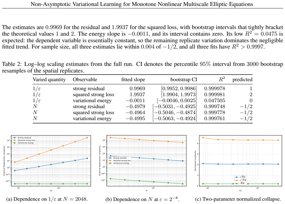
We develop a non-asymptotic approximation, sampling, and finite-iteration optimization theory for variational physics-informed approximation of uniformly monotone nonlinear multiscale elliptic equations. For boundary-compatible neural feature classes, the population error splits into approximation, empirical quadrature, and projected-gradient terms, with all non-approximation constants uniform in the microscopic scale \(\varepsilon\). Assuming a quantitative corrected \(H^1\)-estimate, a two-scale state class yields \[ \mathcal A_m^\varepsilon \le C\bigl(\varepsilon+\Phi_{0,m_0}^2+\Phi_{1,m_1}^2\bigr) \] in arbitrary dimension. We further introduce a convex primal-dual physics loss whose population value is a computable upper certificate for the state error. With additional flux-corrector regularity, a divergence-compatible two-scale flux class gives a certified state-flux bound combining \(O(\varepsilon)\) approximation, state and flux feature errors, empirical sampling error, and an \(O(K^{-1})\) optimization term. In contrast, for general periodic nonlinear fluxes satisfying a natural nondegeneracy condition, the empirical Rademacher complexities of strong-residual and squared-residual classes are bounded below by constant multiples of \((\varepsilon\sqrt N)^{-1}\) and \((\varepsilon^2\sqrt N)^{-1}\), respectively. These optimizer-independent lower bounds hold in every spatial dimension. Numerical experiments confirm the predicted \(\varepsilon\)- and \(N\)-scalings for nonlinear fluxes in \(d=1,2,3\), validate every computed primal-dual certificate, and show that corrector-enriched classes substantially reduce energy and \(H^1\) errors as the microscopic scale is refined.

Figures

Figures reproduced from arXiv: 2607.15702 by Ronald Katende.

**Figure 2.** Figure 2: Robustness of the strong-form result. Panel (a) tests nonlinear fluxes in dimensions [PITH_FULL_IMAGE:figures/full_fig_p018_2.png] view at source ↗

**Figure 3.** Figure 3: Numerical validation of the primal–dual theory. Panel (a) verifies the reliability inequality; panel (b) shows [PITH_FULL_IMAGE:figures/full_fig_p018_3.png] view at source ↗

discussion (0)

Reference graph

Works this paper leans on

11 extracted references · 2 canonical work pages

[1]

Estimates on the generalization error of physics-informed neural networks for approximating pdes

Siddhartha Mishra and Roberto Molinaro. Estimates on the generalization error of physics-informed neural networks for approximating pdes. IMA Journal of Numerical Analysis, 43 0 (1): 0 1--43, 2023. doi:10.1093/imanum/drab093

doi:10.1093/imanum/drab093 2023
[2]

The deep ritz method: A deep learning-based numerical algorithm for solving variational problems

Weinan E and Bing Yu. The deep ritz method: A deep learning-based numerical algorithm for solving variational problems. Communications in Mathematics and Statistics, 6 0 (1): 0 1--12, 2018. doi:10.1007/s40304-018-0127-z

doi:10.1007/s40304-018-0127-z 2018
[3]

Variational physics-informed neural networks for solving partial differential equations

Ehsan Kharazmi, Zhongqiang Zhang, and George Em Karniadakis. Variational physics-informed neural networks for solving partial differential equations. arXiv preprint arXiv:1912.00873, 2019

Pith/arXiv arXiv 1912
[4]

Arnav Gangal, Luis Kim, and Sean P. Carney. Physics-informed neural networks for elliptic equations with oscillatory differential operators. arXiv preprint arXiv:2212.13531, 2023

Pith/arXiv arXiv 2023
[5]

Correctors for the homogenization of monotone operators

Gianni Dal Maso and Anneliese Defranceschi. Correctors for the homogenization of monotone operators. Differential and Integral Equations, 3 0 (6): 0 1151--1166, 1990

1990
[6]

Correctors for some nonlinear monotone operators

Johan Bystr \"o m. Correctors for some nonlinear monotone operators. Journal of Nonlinear Mathematical Physics, 8 0 (1): 0 8--30, 2001. doi:10.2991/jnmp.2001.8.1.2

work page doi:10.2991/jnmp.2001.8.1.2 2001
[7]

Quantitative estimates on periodic homogenization of nonlinear elliptic operators

Li Wang, Qiang Xu, and Peihao Zhao. Quantitative estimates on periodic homogenization of nonlinear elliptic operators. arXiv preprint arXiv:1807.10865, 2018

Pith/arXiv arXiv 2018
[8]

Primal-dual gap estimators for a posteriori error analysis of nonsmooth minimization problems

S \"o ren Bartels and Marijo Milicevic. Primal-dual gap estimators for a posteriori error analysis of nonsmooth minimization problems. ESAIM: Mathematical Modelling and Numerical Analysis, 54 0 (5): 0 1635--1660, 2020. doi:10.1051/m2an/2019074

arXiv 2020
[9]

A priori error estimate of deep mixed residual method for elliptic PDEs

Lingfeng Li, Xue-Cheng Tai, Jiang Yang, and Quanhui Zhu. A priori error estimate of deep mixed residual method for elliptic PDEs . Journal of Scientific Computing, 98 0 (2): 0 44, 2024. doi:10.1007/s10915-023-02432-x

work page doi:10.1007/s10915-023-02432-x 2024
[10]

Bersetche and Juan Pablo Borthagaray

Francisco M. Bersetche and Juan Pablo Borthagaray. A deep first-order system least squares method for solving elliptic PDEs . Computers & Mathematics with Applications, 129: 0 136--150, 2023. doi:10.1016/j.camwa.2022.11.014

doi:10.1016/j.camwa.2022.11.014 2023
[11]

Joost A. A. Opschoor, Philipp C. Petersen, and Christoph Schwab. First order system least squares neural networks. arXiv preprint arXiv:2409.20264, 2024

Pith/arXiv arXiv 2024

[1] [1]

Estimates on the generalization error of physics-informed neural networks for approximating pdes

Siddhartha Mishra and Roberto Molinaro. Estimates on the generalization error of physics-informed neural networks for approximating pdes. IMA Journal of Numerical Analysis, 43 0 (1): 0 1--43, 2023. doi:10.1093/imanum/drab093

doi:10.1093/imanum/drab093 2023

[2] [2]

The deep ritz method: A deep learning-based numerical algorithm for solving variational problems

Weinan E and Bing Yu. The deep ritz method: A deep learning-based numerical algorithm for solving variational problems. Communications in Mathematics and Statistics, 6 0 (1): 0 1--12, 2018. doi:10.1007/s40304-018-0127-z

doi:10.1007/s40304-018-0127-z 2018

[3] [3]

Variational physics-informed neural networks for solving partial differential equations

Ehsan Kharazmi, Zhongqiang Zhang, and George Em Karniadakis. Variational physics-informed neural networks for solving partial differential equations. arXiv preprint arXiv:1912.00873, 2019

Pith/arXiv arXiv 1912

[4] [4]

Arnav Gangal, Luis Kim, and Sean P. Carney. Physics-informed neural networks for elliptic equations with oscillatory differential operators. arXiv preprint arXiv:2212.13531, 2023

Pith/arXiv arXiv 2023

[5] [5]

Correctors for the homogenization of monotone operators

Gianni Dal Maso and Anneliese Defranceschi. Correctors for the homogenization of monotone operators. Differential and Integral Equations, 3 0 (6): 0 1151--1166, 1990

1990

[6] [6]

Correctors for some nonlinear monotone operators

Johan Bystr \"o m. Correctors for some nonlinear monotone operators. Journal of Nonlinear Mathematical Physics, 8 0 (1): 0 8--30, 2001. doi:10.2991/jnmp.2001.8.1.2

work page doi:10.2991/jnmp.2001.8.1.2 2001

[7] [7]

Quantitative estimates on periodic homogenization of nonlinear elliptic operators

Li Wang, Qiang Xu, and Peihao Zhao. Quantitative estimates on periodic homogenization of nonlinear elliptic operators. arXiv preprint arXiv:1807.10865, 2018

Pith/arXiv arXiv 2018

[8] [8]

Primal-dual gap estimators for a posteriori error analysis of nonsmooth minimization problems

S \"o ren Bartels and Marijo Milicevic. Primal-dual gap estimators for a posteriori error analysis of nonsmooth minimization problems. ESAIM: Mathematical Modelling and Numerical Analysis, 54 0 (5): 0 1635--1660, 2020. doi:10.1051/m2an/2019074

arXiv 2020

[9] [9]

A priori error estimate of deep mixed residual method for elliptic PDEs

Lingfeng Li, Xue-Cheng Tai, Jiang Yang, and Quanhui Zhu. A priori error estimate of deep mixed residual method for elliptic PDEs . Journal of Scientific Computing, 98 0 (2): 0 44, 2024. doi:10.1007/s10915-023-02432-x

work page doi:10.1007/s10915-023-02432-x 2024

[10] [10]

Bersetche and Juan Pablo Borthagaray

Francisco M. Bersetche and Juan Pablo Borthagaray. A deep first-order system least squares method for solving elliptic PDEs . Computers & Mathematics with Applications, 129: 0 136--150, 2023. doi:10.1016/j.camwa.2022.11.014

doi:10.1016/j.camwa.2022.11.014 2023

[11] [11]

Joost A. A. Opschoor, Philipp C. Petersen, and Christoph Schwab. First order system least squares neural networks. arXiv preprint arXiv:2409.20264, 2024

Pith/arXiv arXiv 2024