REVIEW 2 major objections 5 minor 1 cited by
Phase field approximation for Plateau's problem: a curve geodesic distance penalty approach
T0 review · 2 major / 5 minor · reviewed 2026-08-06 · deepseek-v4-flash
Pith's one-line read For a single Lipschitz curve on a cylinder's edge, quasi-minimizers of an Ambrosio-Tortorelli energy with a geodesic distance penalty converge to a Plateau minimal surface.
desk verdict The model is a real step toward phase-field Plateau approximations, and the cylinder-case Gamma-convergence proof is mostly sound, but the p<∞ branch has a genuine Chebyshev gap that leaves Theorem 1.1 unproved for the numerically relevant p=2; the fix is easy, so it deserves peer review. read the letter →
The pith
A machine-rendered reading of the paper's core claim, the machinery that carries it, and where it could break.
The reading
What carries the argument
The central object is the functional $F^p_\varepsilon(u)=\varepsilon\int_C|\nabla u|^2\,dx+\frac{1}{4\varepsilon}\int_C(1-u)^2\,dx+\frac{1}{c_\varepsilon}d^p_u(\gamma,\gamma_0)$, where $d^p_u$ is the $p$-geodesic distance between curves, defined as the infimum of $\int_{S_\ell}(|u|^p+\delta_\varepsilon)\,dH^2$ (or of the sup norm when $p=\infty$) over Lipschitz homotopies $\ell$ joining $\gamma$ to $\gamma_0$, with $S_\ell=\ell([0,1]\times S^1)$. The geodesic term is the carrier of the topological constraint: when it is small, the surface $S_\ell$ lies in a region where $u$ is small, and the separation property of such surfaces forces the selected level set to separate the cylinder. The proof then uses the co-area formula on $g_\varepsilon=u_\varepsilon-u_\varepsilon^2/2$, an averaging lemma to pick a good level $t_\varepsilon$, and the two competitors extracted from the separated components to obtain the liminf bound.
What would settle it
Run the numerical scheme in the exact one-curve cylinder setting and measure the perimeter in $C_0$ of the $L^1$ limit of the selected level-set component; if for a quasi-minimizing sequence that perimeter is strictly larger than the perimeter of the graph minimizer, Theorem 1.1 fails. A more targeted check is whether the Minkowski content identity $\lim_{r\to0}\mathcal{L}^3(K_r)/(2r)=H^2(K)$ holds for the essential boundary $K$ of the cylinder minimizer; a violation there breaks the limsup construction.
Extended reading notes
Core claim
The central claim is Theorem 1.1: for $p\in[1,\infty]$, if the prescribed curve $\gamma$ is the graph of a Lipschitz function on the lateral boundary of a cylinder and $\gamma_0$ is a constant curve inside it, then any quasi-minimizing sequence $u_\varepsilon$ of $F^p_\varepsilon$ yields a level set $\{u_\varepsilon-u_\varepsilon^2/2>t_\varepsilon\}$ whose component containing the upper part of the cylinder converges in $L^1$, up to a subsequence, to a solution of Plateau's problem. The proof is a $\Gamma$-convergence style argument: the limsup inequality builds a recovery sequence from the optimal Modica-Mortola profile around the minimizer's boundary, while the liminf inequality selects a suitable level set, proves it separates the cylinder, and reads off two competitors whose perimeters force the limit to be minimal. The paper therefore claims that topology can be prescribed by a penalty term at the limit, removing the need for an explicit current or divergence constraint.
Load-bearing premise
The proof depends on the regularity of the ideal minimal surface: its boundary is a graph, its essential boundary coincides with its topological boundary almost everywhere, and its area in small balls is bounded above and below by a constant times the radius squared; if that regularity fails, the recovery sequence used in the limsup inequality may not have the claimed energy.
Editorial extensions
If this is right
- Quasi-minimizers of $F^p_\varepsilon$ give a computable route to least-area surfaces: minimizers of the phase field energy approximate Plateau solutions without imposing a divergence or current constraint on the field.
- In the cylinder setting, any algorithm that decreases the energy sufficiently fast eventually produces the minimal surface, because the energy gap to the optimum controls the $L^1$ distance of the selected level-set component.
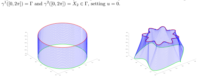
- The same geodesic-penalty design extends formally to several boundary curves and to non-oriented films, as the numerical experiments with catenoids, tubes, and the cube suggest.
- The method is a higher-dimensional analogue of the Steiner phase field approximation: shortest connection between points is replaced by least-area homotopy between curves.
Reading between the lines
- The cylinder and single-curve assumptions look technical rather than essential; a natural conjecture is that the same level-set argument works on any domain where admissible homotopies separate the boundary and the limit minimizer is Ahlfors regular up to the boundary.
- The numerical construction uses non-optimal geodesics and still converges to good films, which suggests the geodesic penalty is doing less topological work than the analysis requires; testing the exact energy with optimal geodesics in the cylinder would isolate how much slack the numerical relaxation introduces.
- The choice of connection graph $I_\gamma$ (which curve is paired with which point or curve) appears to select which Plateau solution is reached, so variants that learn $I_\gamma$ during the flow could target or avoid singular solutions such as the tube connecting two disks.
- Proving a $\Gamma$-limit for the Willmore-Cahn-Hilliard variant and for multiple curves would close the gap between the analysis and the numerics; numerical benchmarks with measured perimeters could serve as the first evidence.
Editorial analysis
A structured set of objections, weighed in public.
Referee Report
Summary. The paper proposes a phase-field approximation of a Reifenberg-type Plateau problem in R^3. The functional combines an Ambrosio-Tortorelli term with a p-geodesic distance penalty between a prescribed boundary curve and a point on it, generalizing earlier Steiner-problem approximations. The main theoretical result, Theorem 1.1, states that in a cylinder, for p in [1,∞], any quasi-minimizing sequence of the p-energy produces level sets that converge in L1 to a solution of the Plateau problem. The proof is organized as a Γ-limsup/liminf pair (Theorems 2.1 and 2.2), with the liminf proof using a separation argument based on the Borsuk theorem and an averaging argument over level sets. The numerical section develops a gradient-flow scheme using a Willmore-Cahn-Hilliard variant and fast-marching approximations of the geodesic term, with experiments for one, two, three, and six boundary curves, including the cube example.
Significance. If the main theorem is correct, this is a valuable contribution: it provides a new phase-field model for Plateau's problem in the Reifenberg sense, with a topological penalty that is not reduced to a current boundary constraint, and it gives the first Γ-convergence analysis in a nontrivial geometric setting. The proof is genuinely original in its use of separation and level-set averaging, and no fitted parameters or circular arguments are involved. The numerical experiments are visually convincing and suggest that the model is practically useful. However, the manuscript currently contains a load-bearing gap in the p<∞ part of the liminf proof, and it depends at a central point on an unpublished regularity result. These issues need to be resolved before the claims can be accepted as stated.
major comments (2)
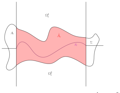
- [§2.5.3, Step 2 (Eq. (28))] The Chebyshev bound displayed in Step 2 is not a consequence of the energy estimate. From ∫_{S_ℓε} |uε|^p dH² ≤ C cε one obtains H²(S_ℓε ∩ {uε ≥ α}) ≤ C cε / α^p, not (C cε/α)^p as written. With the chosen αε = √cε, the correct bound gives H²(Kε) ≤ C cε^{1−p/2}, which fails to tend to zero for p ≥ 2 and diverges for p > 2. Consequently assertion (28), the conclusion P(Uε) → 0, and equality (31) in Step 3 are not established for p ∈ [2,∞), which includes the value p = 2 used throughout the numerical section. The gap appears repairable, for example by taking αε = cε^{1/(2p)}, which gives H²(Kε) = O(√cε) and still sε → 0; but as written the p<∞ half of Theorem 2.2, and hence Theorem 1.1, is incomplete.
- [Proposition 2.1, used in §2.4 (Eq. (13)) and §2.5] The limsup inequality relies on the Ahlfors regularity of the essential boundary through (12)–(13), while the liminf proof uses the graph structure and the equality ∂∗Ω = ∂Ω stated in Proposition 2.1. The proof of this proposition is not contained in the manuscript; it is attributed to the unpublished manuscript [Mac25] ('in preparation'). Since these properties are load-bearing for both inequalities, the paper is not self-contained at a central point. The authors should provide a proof of Proposition 2.1, or at least a detailed self-contained argument in an appendix, or replace the reference by a publicly available verifiable source.
minor comments (5)
- [§2.4, Eq. (15)] In the p<∞ part of the limsup proof, the integral of |uε|^p over K equals H²(K)(kε^p + δε), not H²(K)(kε + δε) as displayed; the conclusion (15) is unchanged because kε = cε² makes the extra factor vanish, but the displayed equality is inaccurate.
- [§2.5.2, Step 4, Eq. (22)] The displayed identity '∂∗Ω1ε ∩ ∂∗Ω1ε ∩ C0 = ∅' should almost certainly read '∂∗Ω1ε ∩ ∂∗Ω2ε ∩ C0 = ∅'.
- [Theorem 1.1] The statement asserts sε = O(cε), but in the p<∞ proof sε = αε − αε²/2 with αε = √cε (and after the proposed fix, αε = cε^{1/(2p)}); in neither case is sε = O(cε) for p ≥ 2. The theorem should state sε → 0, or give the exact order.
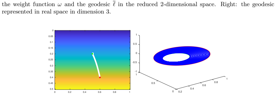
- [§3.2, numerical experiments] The numerical section explicitly acknowledges (Remark 3.3 and §3.2.2) that the computed geodesics are not optimal and reports no quantitative error metrics; the cylinder-instead-of-catenoid example is admitted. The numerical claims are therefore qualitative, and the paper should add convergence or error data, or state more cautiously that these are heuristic illustrations.
- [§3.1.2] The statement that replacing ATε by the Willmore-Cahn-Hilliard energy Pε preserves the Γ-convergence result is made without proof or reference; since the numerical minimization uses Pε, a precise statement or reference would be helpful.
Circularity Check
No circularity: the claimed Gamma-limit is derived from the functional's own construction; the only load-bearing external input is a regularity proposition, and the noted p<infinity gap is a correctness issue rather than a reduction to inputs.
full rationale
The derivation chain is not circular. The functional F^p_epsilon is defined by an Ambrosio-Tortorelli term plus a geodesic-distance penalty (Definition 1.1 and equation (6)), and the claimed Gamma-limits (Theorems 2.1 and 2.2) are proved by explicit recovery sequences and coarea/perimeter estimates. No parameter is fitted to the target perimeter, and the geodesic-distance upper bound in the limsup is computed on the actual graph minimizer supplied by Proposition 2.1 rather than imposed by construction. The main external input, Proposition 2.1, is cited partly to [Mac25], an in-preparation manuscript by one of the authors, but that proposition is a regularity statement for Plateau minimizers whose hypotheses do not mention the phase-field model or geodesic penalty; under the stated criteria this is load-bearing but independent support, not circularity. A separate correctness gap should be flagged: in Section 2.5.3, Step 2, the choice alpha_epsilon = sqrt(c_epsilon) gives, by Chebyshev, H^2(K_epsilon) <= C c_epsilon^{1-p/2}, which does not tend to 0 for p >= 2, so assertion (28) is unjustified. This is an incompleteness in the p < infinity branch of Theorem 2.2, not an instance of a claimed result being equivalent to its inputs. The numerics use p = 2 and are explicitly outside the proved setting, so they do not create circular validation either. Overall, no step reduces a claimed prediction to its input by definition or by fitting.
Assumptions & free parameters
free parameters (9)
- c_epsilon =
converges to 0, with delta_epsilon/c_epsilon -> 0
- delta_epsilon =
converges to 0
- k_epsilon =
c_epsilon^2
- alpha_epsilon =
sqrt(c_epsilon) as written
- spatial grid size P =
2^7
- interface width epsilon =
2/P
- time step delta_t =
10 epsilon^2
- Willmore weight sigma_epsilon =
1/epsilon^2
- kernel size r =
0.1 epsilon^2
assumptions (5)
- domain assumption Existence of a Plateau minimizer that is open with ∂*Omega=∂Omega H2-a.e. and Ahlfors regular up to the boundary (Proposition 2.1).
- standard math Rado's theorem: a Jordan curve with one-to-one orthogonal projection onto a convex curve has a unique minimal surface solution that is a graph.
- standard math Borsuk separation theorem: if a compact set A is deformed into B without crossing p,q, then p,q remain in distinct components.
- standard math Coarea formula for BV and for Lipschitz functions, and the average-value lemma for finite measures.
- domain assumption The prescribed curve Gamma is a Lipschitz graph over S1 and gamma0 is a constant curve at a point of Gamma.
Cite this review
Pith. "Pith review of Phase field approximation for Plateau's problem: a curve geodesic distance penalty approach." pith.science (2026). https://pith.science/paper/T36375YC
@misc{pith2026250622273,
  author       = {Pith},
  title        = {Pith review of: Phase field approximation for Plateau's problem: a curve geodesic distance penalty approach},
  year         = {2026},
  howpublished = {\url{https://pith.science/paper/T36375YC}},
  note         = {Machine review of arXiv:2506.22273}
}
read the original abstract
This work focuses on a phase field approximation of Plateau's problem. Inspired by Reifenberg's point of view, we introduce a model that combines the Ambrosio-Torterelli energy with a geodesic distance term, which can be considered as a generalization of the approach developed by Bonnivard, Lemenant and Santambrogio to approximate solutions to Steiner's problem. First, we present a Gamma-convergence analysis of this model in the simple case of a single curve located on the edge of a cylinder. In a numerical section, we detail the numerical optimisation schemes used to minimize this energy for numerous examples, for which good approximations of solutions to Plateau's problem are found.
Figures


Figures from the paper (15 more)





Forward citations
Cited by 1 Pith paper
-
Optimal regularity up to the boundary for Plateau-quasi-minimizers
Plateau-quasi-minimizers in co-dimension one are characterized, up to the boundary, by bi-John domains with Ahlfors regular boundaries.
Reference graph
Works this paper leans on
-
[1]
Ambrosio, N
L. Ambrosio, N. Fusco, and D. Pallara. Functions of bounded variation and free discontinuity problems . Oxford Mathematical Monographs. The Clarendon Press, Oxford University Press, New York, 2000
2000
-
[2]
M. Bonnivard, E. Bretin, and A. Lemenant. Numerical approximation of the Steiner problem in dimension 2 and 3 . Math. Comput. , 89(321):1--43, 2020
work page 2020
-
[3]
A cahn--hilliard--willmore phase field model for non-oriented interfaces, 2024
Elie Bretin, Antonin Chambolle, and Simon Masnou. A cahn--hilliard--willmore phase field model for non-oriented interfaces, 2024
work page 2024
-
[4]
A penalized allen-cahn equation for the mean curvature flow of thin structures, 2024
Elie Bretin, Chih-Kang Huang, and Simon Masnou. A penalized allen-cahn equation for the mean curvature flow of thin structures, 2024
work page 2024
-
[5]
Matthieu Bonnivard, Antoine Lemenant, and Vincent Millot. On a phase field approximation of the planar steiner problem: existence, regularity, and asymptotic of minimizers. Interfaces and free Boundaries , 20(1):69--106, 2018
work page 2018
-
[6]
M. Bonnivard, A. Lemenant, and F. Santambrogio. Approximation of length minimization problems among compact connected sets. SIAM Journal on Mathematical Analysis , 47(2):1489--1529, 2015
work page 2015
-
[7]
A numerical method for computing minimal surfaces in arbitrary dimension
Thomas Cecil. A numerical method for computing minimal surfaces in arbitrary dimension. J. Comput. Phys. , 206(2):650--660, 2005
work page 2005
-
[8]
Antonin Chambolle, Luca A. D. Ferrari, and Benoit Merlet. Variational approximation of size-mass energies for \(k\) -dimensional currents. ESAIM, Control Optim. Calc. Var. , 25:39, 2019. Id/No 43
work page 2019
Show all 38 references
-
[9]
A phase-field approximation of the Steiner problem in dimension two
Antonin Chambolle, Luca Alberto Davide Ferrari, and Benoit Merlet. A phase-field approximation of the Steiner problem in dimension two. Adv. Calc. Var. , 12(2):157--179, 2019
2019
-
[10]
Coppin and D
C. Coppin and D. Greenspan. A contribution to the particle modeling of soap films. Appl. Math. Comput. , 26(4):315--331, 1988
1988
-
[11]
David L. Chopp. Computing minimal surfaces via level set curvature flow. J. Comput. Phys. , 106(1):77--91, 1993
1993
-
[12]
G. David. Sliding almost minimal sets and the Plateau problem. In Harmonic analysis and applications , pages 199--256. Providence, RI: American Mathematical Society (AMS); Princeton, NJ: Institute for Advanced Study (IAS), 2020
2020
-
[13]
Su una teoria generale della misura \((r-1)\) -dimensionale in uno spazio ad \(r\) dimensioni
Ennio De Giorgi. Su una teoria generale della misura \((r-1)\) -dimensionale in uno spazio ad \(r\) dimensioni. Ann. Mat. Pura Appl. (4) , 36:191--213, 1954
1954
-
[14]
Frontiere orientate di misura minima
Ennio De Giorgi. Frontiere orientate di misura minima. Seminario di Matematica. Scuola Normale Superiore di Pisa , 1960
1960
-
[15]
Hutchinson
Gerhard Dziuk and John E. Hutchinson. The discrete P lateau problem: algorithm and numerics. Math. Comp. , 68(225):1--23, 1999
1999
-
[16]
Hutchinson
Gerhard Dziuk and John E. Hutchinson. The discrete P lateau problem: convergence results. Math. Comp. , 68(226):519--546, 1999
1999
-
[17]
A direct approach to plateau's problem
Camillo De Lellis, Francesco Ghiraldin, and Francesco Maggi. A direct approach to plateau's problem. Journal of the European Mathematical Society , 19(8):2219--2240, 2017
2017
-
[18]
A method of numerical solution of the problem of P lateau
Jesse Douglas. A method of numerical solution of the problem of P lateau. Ann. of Math. (2) , 29(1-4):180--188, 1927/28
1927
-
[19]
Dugundji
J. Dugundji. Topology . Allyn and Bacon series in advanced mathematics. Allyn and Bacon, 1966
1966
-
[20]
L.C Evans and R.F. Gariepy. Measure Theory and Fine Properties of Functions . Studies in Advanced Mathematics. Taylor and Francis , 1991
1991
-
[21]
D. Eyre. Computational and mathematical models of microstructural evolution. Warrendale:The Material Research Society , 1998
1998
-
[22]
Herbert Federer and Wendell H. Fleming. Normal and integral currents. Annals of Mathematics , 72(3):458--520, 1960
1960
-
[23]
Minimal surfaces and functions of bounded variation , volume 80 of Monogr
Enrico Giusti. Minimal surfaces and functions of bounded variation , volume 80 of Monogr. Math., Basel . Birkh \"a user, Cham, 1984
1984
-
[24]
Soap film solutions to plateau’s problem
Jenny Harrison. Soap film solutions to plateau’s problem. Journal of Geometric Analysis , 24:271--297, 2014
2014
-
[25]
Existence and soap film regularity of solutions to plateau’s problem
Jenny Harrison and Harrison Pugh. Existence and soap film regularity of solutions to plateau’s problem. Advances in Calculus of Variations , 9(4):357--394, 2016
2016
-
[26]
Blaine jun
H. Blaine jun. Lawson. Lectures on minimal submanifolds. Vol . I , volume 9 of Math. Lect. Ser. Publish or Perish, Inc., Wilmington, 1980
1980
-
[27]
A Modica - Mortola approximation for the Steiner problem
Antoine Lemenant and Filippo Santambrogio. A Modica - Mortola approximation for the Steiner problem. C. R., Math., Acad. Sci. Paris , 352(5):451--454, 2014
2014
-
[28]
Machefert
E. Machefert. Optimal regularity up to the boundary for plateau-quasi-minimizers. in preparation , 2025
2025
-
[29]
Sets of finite perimeter and geometric variational problems
Francesco Maggi. Sets of finite perimeter and geometric variational problems. An introduction to geometric measure theory , volume 135 of Camb. Stud. Adv. Math. Cambridge: Cambridge University Press, 2012
2012
-
[30]
A hierarchy of plateau problems and the approximation of plateau's laws via the allen--cahn equation
Francesco Maggi, Michael Novack, and Daniel Restrepo. A hierarchy of plateau problems and the approximation of plateau's laws via the allen--cahn equation. arXiv preprint arXiv:2312.11139 , 2023
2023 arXiv
-
[31]
Plateau borders in soap films and gauss' capillarity theory
Francesco Maggi, Michael Novack, and Daniel Restrepo. Plateau borders in soap films and gauss' capillarity theory. arXiv preprint arXiv:2310.20169 , 2023
2023 arXiv
-
[32]
On the problem of Plateau , volume 2 of Ergeb
Tibor Rad \'o . On the problem of Plateau , volume 2 of Ergeb. Math. Grenzgeb. Springer-Verlag, Berlin, 1933
1933
-
[33]
E. R. Reifenberg. Solution of the Plateau problem for \(m\) -dimensional surfaces of varying topological type. Acta Math. , 104:1--92, 1960
1960
-
[34]
J. A. Sethian. Fast marching methods. SIAM Review , 41(2):199--235, 1999
1999
-
[35]
J. A. Sethian. Level Set Methods and Fast Marching Methods . Cambridge University Press, second edition edition, 1999
1999
-
[36]
J. Shen, C. Wang, X. Wang, and S. M. Wise. Second-order convex splitting schemes for gradient flows with E hrlich- S chwoebel type energy: Application to thin film epitaxy. SIAM J. Numerical Analysis , 50(1):105--125, 2012
2012
-
[37]
H.-J. Wagner. A contribution to the numerical approximation of minimal surfaces. Computing , 19(1):35--58, 1977/78
1977
-
[38]
Computing minimal surfaces with differential forms
Stephanie Wang and Albert Chern. Computing minimal surfaces with differential forms. ACM Trans. Graph. , 40(4):113:1--113:14, August 2021
2021
Reviewed August 6, 2026 · model on record in the stance chip above.
Discussion (0). Continue with ORCID to comment.