REVIEW 4 major objections 4 minor 47 references
Augmented NETT Regularization of Inverse Problems
T0 review · 4 major / 4 minor · reviewed 2026-08-14 · deepseek-v4-flash
Pith's one-line read aNETT regularization adds an autoencoder consistency penalty to the NETT functional, proving coercivity of the regularizer and yielding stability, convergence, and an O(ε) convergence rate for finite-rank forward operators.
desk verdict aNETT is a genuine and mostly well-proved extension of NETT, but the abstract overclaims on computational cost and the numerical scheme sits outside the theory. read the letter →
The pith
A machine-rendered reading of the paper's core claim, the machinery that carries it, and where it could break.
The reading
What carries the argument
The carrying object is the aNETT regularizer $R(x)=Q(E(x))+(c/2)\|x-(D\circ E)(x)\|^2$, where $E$ is an encoder into $\ell^2$, $D$ a decoder, $Q$ a coercive complexity penalty, and $c>0$. The second term penalizes the distance from $x$ to the autoencoder output, forcing reconstructions to stay near the learned signal manifold. Its role in the proofs is to supply coercivity: combining $Q$'s coercivity with weak sequential continuity of $D$, the inequality $\|x_n\| \le 2\|x_n-(D\circ E)(x_n)\|^2+2\|(D\circ E)(x_n)\|^2$ bounds every sequence on which $R$ is bounded; coercivity then drives the existence, stability, and convergence theorems. The practical minimization is carried out by an ADMM scheme whose encoder update is a proximal step for $Q$, which is a soft-thresholding step for the $\ell^1$ penalty.
What would settle it
Take a weakly convergent, non-strongly-convergent sequence of images (for example, unit-amplitude sine waves with frequency tending to infinity) and evaluate the trained aNETT regularizer $R$ on it; if $R$ stays bounded while the images do not converge strongly, coercivity fails, and minimizers of the aNETT functional may fail to exist. Alternatively, compute aNETT reconstructions on a fixed inverse problem at increasing discretization resolutions; if the regularizer value or reconstruction error blows up as the grid refines, the infinite-dimensional assumptions are not satisfied by the implementation.
Extended reading notes
Core claim
The central claim is that adding the term $(c/2)\|x-(D\circ E)(x)\|^2$ to the NETT regularizer converts a data-driven regularization scheme that needed ad-hoc early stopping into one with a full convergence theory. Under Conditions (A1)-(A6), the regularizer $R$ is coercive because boundedness of $Q(E(x_n))$ bounds $E(x_n)$, weak sequential continuity of $D$ bounds $(D\circ E)(x_n)$, and the triangle inequality then bounds $x_n$. This coercivity yields existence of minimizers for every data point, stability in the sense that weak accumulation points of minimizers for perturbed data are minimizers for the exact data, and weak convergence of regularized solutions to $R$-minimizing solutions as $\varepsilon/\alpha$ and $\alpha$ tend to zero; strong convergence follows when $R$ is totally nonlinear. For finite-rank $K$ with Lipschitz Gâteaux-differentiable $R$, the absolute Bregman distance between regularized and exact solutions is $O(\varepsilon)$ under the parameter choice $\alpha\asymp\varepsilon$. The theory is stated for Hilbert spaces and applies as well to any coercive weakly lower semi-continuous regularizer replacing $Q(E)+$ the manifold penalty.
Load-bearing premise
The load-bearing premise is that the encoder $E$ and decoder $D$ are weakly sequentially continuous maps between Hilbert spaces; if a trained network lacks this property, the coercivity proof and the infinite-dimensional convergence theory do not apply to it.
Editorial extensions
If this is right
- aNETT minimizers exist for all noisy data and depend stably on the data, so early stopping is no longer needed as a hidden regularizer.
- With a suitable parameter choice, regularized solutions converge to $R$-minimizing solutions, and in the finite-rank Lipschitz case the error in absolute Bregman distance is $O(\varepsilon)$.
- Because the optimization does not repeatedly apply the forward operator and its adjoint, aNETT remains usable when the forward model is numerically expensive, unlike learned iterative schemes.
- Networks trained on coarsely sampled data can be applied at higher sampling rates without retraining, and the reconstructions improve with the added measurements.
- The convergence results transfer to any coercive, weakly lower semi-continuous regularizer, not only the specific autoencoder construction.
Reading between the lines
- Because aNETT training never uses the forward operator during the autoencoder step, a natural testable extension is to transfer the same learned regularizer across imaging modalities (for example, from CT to MRI) and compare reconstruction quality.
- The $O(\varepsilon)$ rate is proven for finite-rank $K$; for infinite-dimensional operators such as the continuous Radon transform, a plausible extension is to derive source-condition-dependent rates using the same absolute-Bregman machinery.
- The universality experiment suggests a practical use case in dynamic imaging, where the measurement geometry changes from frame to frame; one could evaluate aNETT on a sequence of sampling patterns without retraining.
- A concrete stress test of the theory is to measure $R$ on weakly-but-not-strongly convergent sequences; if bounded $R$-values occur with unbounded image norms, the coercivity assumptions fail for that architecture.
Signed reviews
Editorial analysis
A structured set of objections, weighed in public.
Referee Report
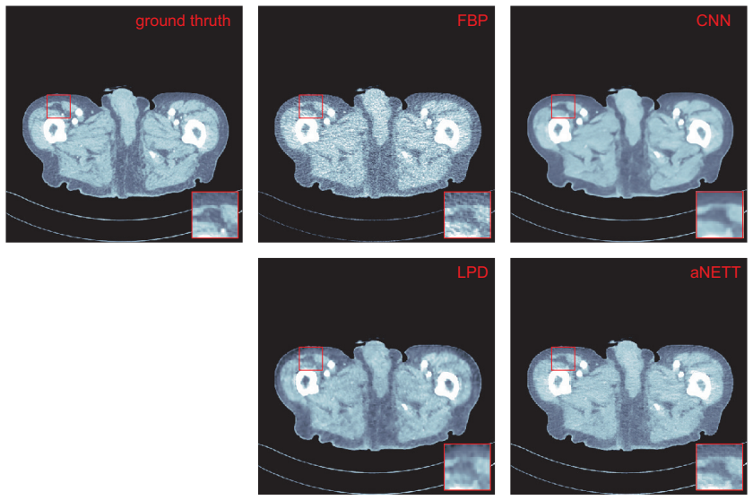
Summary. The paper introduces augmented NETT (aNETT) regularization for inverse problems, defined by the regularizer R(x) = Q(E(x)) + (c/2)||x - (D∘E)(x)||^2, where E is an encoder and D a decoder. The main theoretical contribution is a proof that this regularizer is coercive under weak sequential continuity of E and D and coercivity/weak lower semicontinuity of Q, without explicit coercivity assumptions on the networks. From this coercivity the authors derive existence of minimizers, stability with respect to data perturbation (Theorem 2.6), weak convergence to R-minimizing solutions (Theorem 2.9), strong convergence under total nonlinearity (Theorem 2.12), and convergence rates, including an order-ε rate for finite-rank forward operators with Lipschitz R (Theorem 2.14). The paper also proposes a modular two-stage training strategy and an ADMM-based minimization scheme, and reports numerical comparisons on sparse-view and low-dose CT showing that aNETT is competitive with learned primal-dual and post-processing U-Net methods, with an additional 'universality' experiment at an increased sampling rate without retraining.
Significance. If the main claims hold, aNETT is a valuable contribution to the learned-regularizer literature: it adds a manifold-penalty term that yields coercivity under comparatively mild network assumptions, and it provides a fairly complete regularization-theoretic package (existence, stability, convergence, rates). The proof of coercivity is simple and elegant, and the emphasis on a general similarity measure is a strength. The modular training strategy and the universality experiment address practically relevant issues. However, as detailed below, the advertised practical advantage regarding expensive forward models is contradicted by the proposed algorithm, the numerical solver is not covered by the theory, and the proof of the convergence-rate result contains a logical gap. These issues are repairable, but they currently weaken the central claims.
major comments (4)
- [Abstract and Section 3.2, update (S1)] The abstract and introduction claim that aNETT 'does not require repeated application of the forward and adjoint models,' which is presented as a key advantage for inverse problems with expensive forward models. This is contradicted by the proposed ADMM implementation. In Section 3.2, subproblem (S1) is D(Kx,y^δ) + (αc/2)||x - N(x)||^2 + (ρ/2)||E(x) - ξ^k + u^k||^2, minimized by gradient descent; for the squared-norm similarity measure the gradient contains K^*(Kx - y^δ), and for the KL divergence it contains K^* applied to a residual. Thus every inner gradient step evaluates K and K^*, and with N_iter = 50 outer iterations and up to 10 inner steps per outer iteration, a single reconstruction evaluates the forward and adjoint operators hundreds of times. The claim should be revised to state that the network itself does not contain the forward model, or an implementation that genuinely avoids repeated forward/adjoint evaluations should be provided.
- [Section 3.2] The convergence theory in Section 2 concerns exact minimizers of A_{α,y}, but the numerical reconstructions are obtained by an ADMM scheme in which subproblem (S1) is solved only approximately (gradient descent with at most 10 iterations and a tolerance of 10^-5), and the authors state that convergence of the ADMM scheme is 'beyond the scope of this work.' No result links the approximate ADMM iterates to the minimizers analyzed in Theorems 2.6, 2.9, and 2.14. This gap should be acknowledged clearly, and ideally the approximate solver should be analyzed or its output validated against the theory in some quantitative way.
- [Proposition 2.13 and Theorem 2.14] The proof of Proposition 2.13 appeals to Theorem 2.12 to conclude that ||x_α^δ - x_z|| ≤ ε for sufficiently small α. However, Theorem 2.12 requires the parameter choice δ_n/α_n → 0, whereas part (b) of Proposition 2.13 and Theorem 2.14 use α ~ δ, so the hypothesis is not satisfied. The rate result is therefore not established as written. In the finite-rank case the inequality (2.5) derived in Theorem 2.14 actually holds globally in x, so the argument can likely be repaired by applying that global inequality directly without invoking Theorem 2.12; the authors should rewrite the proof accordingly. As it stands, this is a load-bearing gap in the convergence-rates claim.
- [Condition 2.1, assumptions (A4)-(A5)] The infinite-dimensional theory assumes that E and D are weakly sequentially continuous maps between Hilbert spaces. Standard convolutional networks built with ReLU-type nonlinearities are generally not weakly sequentially continuous on infinite-dimensional function spaces, and the paper gives no example or verification that its proposed architectures satisfy (A4)-(A5). In the finite-dimensional setting of Section 3, weak sequential continuity is automatic for continuous networks, but the paper does not state this explicitly. The authors should clarify the scope of the theoretical results: either restrict the convergence analysis to the finite-dimensional case where the assumptions are verifiable, or discuss which network architectures satisfy the weak-continuity assumptions in infinite dimensions.
minor comments (4)
- [Example 2.7] In the bullet proving failure of (B4), the text first says 'and therefore (B5) does not hold' but the condition being disproved is (B4); this should be corrected. In the same example, the expression 'D(x,y) = ||x - y_n||^2' should presumably read 'D(x,y) = ||x - y||^2'.
- [Section 3.2, update (S3)] The scaled dual-variable update is written as 'u^{k+1} = u^{k+1} + (E(x^{k+1}) - ξ^{k+1})'; it should be 'u^{k+1} = u^k + (E(x^{k+1}) - ξ^{k+1})'.
- [Section 4.1] The sentence 'The number of angular samples N' is taken 40 for low the dose CT and N' = 1138 for the low dose example' is garbled; the intended statement is presumably that sparse-view CT uses N' = 40 and low-dose CT uses N' = 1138.
- [Proposition 2.13, proof] The displayed chain in the proof contains the expression '= R(x_α^δ) - D(Kx_α^δ,y^δ) - (R(x_α^δ) - D(Kx_α^δ,y^δ))', which cancels identically and appears to be a typographical artifact. In addition, the final inequality is written as 'δ^2 - cαδ√q + c^2α^2q/4', while the preceding line gives a positive cross term '+ cαδ√q'; the sign should be corrected, although the O(δ) conclusion is unaffected.
Circularity Check
No significant circularity: coercivity, stability, and convergence rates are derived from stated assumptions; the cited lemma from prior NETT work is independent support rather than a circular input.
full rationale
The paper's core mathematical claims are self-contained. Theorem 2.2 proves coercivity of the aNETT regularizer directly from Conditions (A1)-(A6): boundedness of R(x_n) gives boundedness of Q(E(x_n)), which by coercivity of Q bounds E(x_n); weak sequential continuity of D then bounds N(x_n), and the triangle-type inequality kx_nk <= 2kx_n-N(x_n)k + 2kN(x_n)k yields the conclusion. The stability and weak-convergence results (Theorems 2.6 and 2.9) follow from the standard minimizing-sequence argument using weak lower semi-continuity and the stated similarity-measure conditions; no quantity is fitted to data and then renamed a prediction. The convergence-rate result (Theorem 2.14) derives the source-type estimate from the R-minimality of x_z, finite rank of K, and Lipschitz continuity of R, rather than importing an unverified ansatz. The only load-bearing citation is [27, Proposition 2.9] used in Theorem 2.12 to go from vanishing absolute Bregman distance to norm convergence; that proposition is a stated, parameter-free lemma from prior work (by overlapping authors) about total nonlinearity, and it does not contain the aNETT target result or any fitted constants, so it counts as independent mathematical support under the stated rules. The paper also flags its own limitation that ADMM-based minimization is slower than compared methods, and there is an internal-consistency tension between the abstract's claim that aNETT avoids repeated forward/adjoint applications and the gradient-descent implementation of step (S1) in Section 3.2, which uses K and K* via the similarity measure; this is a correctness/practicality issue, not circularity, because it does not make any derived result equivalent to its inputs by construction. Overall, no prediction reduces to a fit, no uniqueness claim is imported from the authors' prior work, and no ansatz is smuggled in via citation; aNETT's derivation chain is genuinely self-contained.
Assumptions & free parameters
free parameters (4)
- Regularization parameter alpha =
Sparse view and universality: 1e-4; low dose: 5e-3
- Augmentation weight c =
1e2 for all three scenarios
- ADMM inner step size eta =
5e-1 for sparse view and universality; 1e-3 for low dose
- ADMM outer iteration count N_iter =
50 for sparse view and universality; 20 for low dose
assumptions (7)
- domain assumption E and D are weakly sequentially continuous (Conditions A4-A5).
- domain assumption Q is coercive and weakly sequentially lower semi-continuous (Condition A6).
- domain assumption K is weakly sequentially continuous (Condition A3).
- domain assumption Similarity measure D satisfies conditions (B1)-(B5).
- domain assumption D satisfies the quasi triangle inequality (2.2) for the convergence-rate results.
- domain assumption R is totally nonlinear at R-minimizing solutions for strong convergence.
- domain assumption Source condition (2.5) holds for convergence rates.
Cite this review
Pith. "Pith review of Augmented NETT Regularization of Inverse Problems." pith.science (2026). https://pith.science/paper/T3UYMVUB
@misc{pith2026190803006,
  author       = {Pith},
  title        = {Pith review of: Augmented NETT Regularization of Inverse Problems},
  year         = {2026},
  howpublished = {\url{https://pith.science/paper/T3UYMVUB}},
  note         = {Machine review of arXiv:1908.03006}
}
read the original abstract
We propose aNETT (augmented NETwork Tikhonov) regularization as a novel data-driven reconstruction framework for solving inverse problems. An encoder-decoder type network defines a regularizer consisting of a penalty term that enforces regularity in the encoder domain, augmented by a penalty that penalizes the distance to the data manifold. We present a rigorous convergence analysis including stability estimates and convergence rates. For that purpose, we prove the coercivity of the regularizer used without requiring explicit coercivity assumptions for the networks involved. We propose a possible realization together with a network architecture and a modular training strategy. Applications to sparse-view and low-dose CT show that aNETT achieves results comparable to state-of-the-art deep-learning-based reconstruction methods. Unlike learned iterative methods, aNETT does not require repeated application of the forward and adjoint models, which enables the use of aNETT for inverse problems with numerically expensive forward models. Furthermore, we show that aNETT trained on coarsely sampled data can leverage an increased sampling rate without the need for retraining.
Figures


Figures from the paper (1 more)

Reference graph
Works this paper leans on
- [1]
-
[2]
J. Adler and O. Öktem. Solving ill-posed inverse problems using iterative deep neural networks.Inverse Probl., 33:124007, 2017
work page 2017
-
[3]
J. Adler and O. Öktem. Learned primal-dual reconstruction.IEEE Trans. Med. Imag., 37(6):1322–1332, 2018
work page 2018
-
[4]
H. K. Aggarwal, M. P. Mani, and M. Jacob. MoDL: model-based deep learning architecture for inverse problems.IEEE Trans. Med. Imag., 38(2):394–405, 2018
work page 2018
-
[5]
Discretization of learned NETT regularization for solving inverse problems
S. Antholzer and M. Haltmeier. Discretization of learned NETT regularization for solving inverse problems.arXiv:2011.03627, 2020
work page Pith review arXiv 2011
-
[6]
S. Antholzer, M. Haltmeier, and J. Schwab. Deep learning for photoacoustic to- mography from sparse data.Inverse Probl. Sci. and Eng., 27(7):987–1005, 2018
work page 2018
-
[7]
S. Arridge, P. Maass, O. Öktem, and C.-B. Schönlieb. Solving inverse problems using data-driven models.Acta Numer., 28:1–174, 2019
work page 2019
-
[8]
S.Boyd, N.Parikh, andE.Chu. Distributed optimization and statistical learning via the alternating direction method of multipliers. Now Publishers Inc, 2011
work page 2011
Show all 47 references
-
[9]
S. H. Chan, X. Wang, and O. A. Elgendy. Plug-and-play admm for image restora- tion: Fixed-point convergence and applications. IEEE Trans. Comput. Imag., 3(1):84–98, 2016
2016
-
[10]
J. R. Chang, C.-L. Li, B. Poczos, and B. V. Kumar. One network to solve them all–solving linear inverse problems using deep projection models. InIEEE Inter- national Conference on Computer Vision (ICCV), pages 5889–5898, 2017
2017
-
[11]
Daubechies, M
I. Daubechies, M. Defrise, and C. De Mol. An iterative thresholding algorithm for linear inverse problems with a sparsity constraint. Comm. Pure Appl. Math., 57(11):1413–1457, 2004. 18
2004
-
[12]
Dittmer, T
S. Dittmer, T. Kluth, P. Maass, and D. O. Baguer. Regularization by architecture: A deep prior approach for inverse problems.J. Math. Imaging Vis., 62(3):456– 470, 2020
2020
-
[13]
H. W. Engl, M. Hanke, and A. Neubauer.Regularization of inverse problems, volume 375 ofMathematics and its Applications. Kluwer Academic Publishers Group, Dordrecht, 1996
1996
-
[14]
Gabay and B
D. Gabay and B. Mercier. A dual algorithm for the solution of nonlinear variational problems via finite element approximation.Comput. Math. Appl., 2(1):17–40, 1976
1976
-
[15]
Glowinski and A
R. Glowinski and A. Marroco. Sur l’approximation, par elements finis d’ordre un, et la resolution, par penalisation-dualite, d’une classe de problemes de dirichlet non lineares. RAIRO Anal. Numer., 9:41–76, 1975
1975
-
[16]
Grasmair, M
M. Grasmair, M. Haltmeier, and O. Scherzer. Sparse regularization withl q penalty term. Inverse Probl., 24(5):055020, 2008
2008
-
[17]
Haltmeier and L
M. Haltmeier and L. V. Nguyen. Regularization of inverse problems by neural networks. arXiv:2006.03972, 2020
2006 arXiv
-
[18]
Hammernik, T
K. Hammernik, T. Klatzer, E. Kobler, M. P. Recht, D. K. Sodickson, T. Pock, and F. Knoll. Learning a variational network for reconstruction of accelerated mri data. Magnetic resonance in medicine, 79(6):3055–3071, 2018
2018
-
[19]
Han and J
Y. Han and J. C. Ye. Framing U-Net via deep convolutional framelets: Application to sparse-view CT.IEEE Trans. Med. Imag., 37:1418–1429, 2018
2018
-
[20]
Hauptmann, J
A. Hauptmann, J. Adler, S. R. Arridge, and O. Oktem. Multi-scale learned iterative reconstruction. IEEE Trans. Comput. Imag., page to appear, 2021
2021
-
[21]
K. H. Jin, M. T. McCann, E. Froustey, and M. Unser. Deep convolutional neu- ral network for inverse problems in imaging. IEEE Trans. Image Process., 26(9):4509–4522, 2017
2017
-
[22]
D. P. Kingma and J. Ba. Adam: A method for stochastic optimization, 2014. arXiv:1412.6980
2014 arXiv
-
[23]
Kobler, T
E. Kobler, T. Klatzer, K. Hammernik, and T. Pock. Variational networks: connect- ing variational methods and deep learning. InGerman Conference on Pattern Recognition, pages 281–293. Springer, 2017
2017
-
[24]
Kofler, M
A. Kofler, M. Haltmeier, C. Kolbitsch, M. Kachelrieß, and M. Dewey. A U-Nets cascade for sparse view computed tomography. InInternational Workshop on Machine Learning for Medical Image Reconstruction (MLIMR), pages 91–99. Springer, 2018
2018
-
[25]
Kofler, M
A. Kofler, M. Haltmeier, T. Schaeffter, and C. Kolbitsch. An end-to-end-trainable iterative network architecture for accelerated radial multi-coil 2D cine MR image reconstruction. arXiv:2102.00783, 2021. 19
2021 arXiv
-
[26]
D. Lee, J. Yoo, and J. C. Ye. Deep residual learning for compressed sensing MRI. In IEEE 14th International Symposium on Biomedical Imaging, pages 15–18, 2017
2017
-
[27]
H. Li, J. Schwab, S. Antholzer, and M. Haltmeier. NETT: Solving inverse problems with deep neural networks.Inverse Probl., 36(6):065005, 2020
2020
-
[28]
S. Lunz, O. Öktem, and C.-B. Schönlieb. Adversarial regularizers in inverse prob- lems. InAdvances in Neural Information Processing Systems, pages 8507–8516, 2018
2018
-
[29]
Maier, C
A. Maier, C. Syben, T. Lasser, and C. Riess. A gentle introduction to deep learning in medical image processing.Zeitschrift für Medizinische Physik, 29(2):86–101, 2019
2019
-
[30]
A. K. Maier, C. Syben, B. Stimpel, T. Würfl, M. Hoffmann, F. Schebesch, W. Fu, L. Mill, L. Kling, and S. Christiansen. Learning with known operators reduces maximum error bounds.Nat. Mach. Intell., 1(8):373–380, 2019
2019
-
[31]
M. T. McCann, K. H. Jin, and M. Unser. Convolutional neural networks for inverse problems in imaging: A review.IEEE Signal Process. Mag., 34(6):85–95, 2017
2017
-
[32]
McCollough
C. McCollough. TU-FG-207A-04: overview of the low dose CT grand challenge. Med. Phys., 43(6):3759–3760, 2016
2016
-
[33]
Mukherjee, S
S. Mukherjee, S. Dittmer, Z. Shumaylov, S. Lunz, O. Öktem, and C.-B. Schönlieb. Learned convex regularizers for inverse problems.arXiv:2008.02839, 2020
2008 arXiv
-
[34]
Obmann, L
D. Obmann, L. Nguyen, J. Schwab, and M. Haltmeier. Sparse aNETT for solving inverse problems with deep learning. In2020 IEEE 17th International Sympo- sium on Biomedical Imaging Workshops (ISBI Workshops), pages 1–4, 2020
2020
-
[35]
Obmann, J
D. Obmann, J. Schwab, and M. Haltmeier. Deep synthesis regularization of inverse problems. Inverse Probl., 37(1):015005, 2021
2021
-
[36]
C. Pöschl. Tikhonov regularization with general residual term. PhD thesis, University of Innsbruck, 2008
2008
-
[37]
Rivenson, Y
Y. Rivenson, Y. Zhang, H. Günaydın, D. Teng, and A. Ozcan. Phase recovery and holographic image reconstruction using deep learning in neural networks.Light Sci. Appl., 7(2):17141–17141, 2018
2018
-
[38]
Romano, M
Y. Romano, M. Elad, and P. Milanfar. The little engine that could: Regularization by denoising (red).SIAM J. Imaging Sci., 10(4):1804–1844, 2017
2017
-
[39]
Scherzer, M
O. Scherzer, M. Grasmair, H. Grossauer, M. Haltmeier, and F. Lenzen.Variational methods in imaging, volume 167 ofApplied Mathematical Sciences. Springer, New York, 2009
2009
-
[40]
Schlemper, J
J. Schlemper, J. Caballero, J. V. Hajnal, A. Price, and D. Rueckert. A deep cascade of convolutional neural networks for mr image reconstruction. InProc. Inf. Process. Med. Imaging, pages 647–658. Springer, 2017. 20
2017
-
[41]
Schwab, S
J. Schwab, S. Antholzer, and M. Haltmeier. Deep null space learning for inverse problems: convergence analysis and rates.Inverse Probl., 35(2):025008, 2019
2019
-
[42]
Schwab, S
J. Schwab, S. Antholzer, and M. Haltmeier. Big in Japan: Regularizing networks for solving inverse problems.J. Math. Imaging Vis., 62:445–455, 2020
2020
-
[43]
Ulyanov, A
D. Ulyanov, A. Vedaldi, and V. Lempitsky. Deep image prior. In Proceedings of the IEEE conference on computer vision and pattern recognition, pages 9446–9454, 2018
2018
-
[44]
S. V. Venkatakrishnan, C. A. Bouman, and B. Wohlberg. Plug-and-play priors for model based reconstruction. In 2013 IEEE Global Conference on Signal and Information Processing, pages 945–948. IEEE, 2013
2013
-
[45]
G. Wang. A perspective on deep imaging.IEEE Access, 4:8914–8924, 2016
2016
-
[46]
Y. Wang, W. Yin, and J. Zeng. Global convergence of ADMM in nonconvex nonsmooth optimization. Journal of Scientific Computing, 78(1):29–63, 2019
2019
-
[47]
Y. Yang, J. Sun, H. Li, and Z. Xu. Deep ADMM-net for compressive sensing MRI. InProc. 30th International Conference on Neural Information Process- ing Systems, pages 10–18, 2016. 21
2016
Reviewed August 14, 2026 · model on record in the stance chip above.
Discussion (0). Continue with ORCID to comment.