Designing Robust Software Sensors for Nonlinear Systems via Neural Networks and Adaptive Sliding Mode Control

Ayoub Farkane; Mohamed Boutayeb; Mounir Ghogho; Mustapha Oudani

REVIEW 5 major objections 5 minor 32 references

Designing Robust Software Sensors for Nonlinear Systems via Neural Networks and Adaptive Sliding Mode Control

T0 review · 5 major / 5 minor · reviewed 2026-08-06 · deepseek-v4-flash

Challenge this review Re-run · record.json Download PDF Read on arXiv ↗ Review JSON

Pith's one-line read This paper claims that a neural network can learn a time-varying observer gain for a general nonlinear discrete-time system, and that coupling this learned gain with an adaptive sliding-mode correction drives the state-estimation error…

desk verdict A useful engineering idea that overclaims its theory: the convergence proof is circular and the training loss suppresses the observer correction. read the letter →

arxiv 2507.06817 v1 pith:T4557L6I submitted 2025-07-09 math.DS cs.LGcs.NEmath.OC

Ayoub Farkane , Mohamed Boutayeb , Mustapha Oudani , Mounir Ghogho This is my paper · ORCID

classification math.DScs.LGcs.NEmath.OC MSC 93B5393C1093D05

keywords nonlinearstateestimationsoftwaresensorneuralnetworkobserveradaptiveslidingmodecontroltime-varyinggainphysics-informedlossLyapunovconvergencethree-tanksystem

verification ladder T0 review T1 audit T2 compute T3 formal

The pith

A machine-rendered reading of the paper's core claim, the machinery that carries it, and where it could break.

The reading

This paper tries to establish a “nearly universal” software sensor: a state observer that works for nonlinear dynamical systems in their most general form, using only sensor outputs and known inputs, without a linearization step or an explicit transformation to a linear system. The proposed observer lets a neural network produce a time-varying gain matrix from the current time, input, and measured output, while an adaptive sliding-mode term corrects the output error. The authors prove that if the network’s approximation of an ideal stabilizing gain decays exponentially and the sliding-mode gain stays above a positive threshold, the estimation error converges exponentially to a bounded region around zero. The payoff would be an observer-design recipe that applies where classical observers struggle, including systems with non-differentiable dynamics and outputs that mix several states, and the training does not require ground-truth state trajectories.

What carries the argument

The load-bearing mechanism is the observer update with three coupled pieces: a multilayer feedforward network with tanh activations outputs the gain matrix $L_k$ from $(t_k,u_k,y_k)$; the adaptive sliding-mode term $\nu_k=-K_k\tanh(y_k-\hat{y}_k)$ with $K_k=K_0+\alpha\|y_k-\hat{y}_k\|^2$ gives a smooth, error-dependent correction whose gain grows with the output error; and a physics-based MSE loss (residual dynamics plus output error plus weight regularization) trains the network without ground-truth state trajectories. In the convergence proof, the key identity is the error recursion $e_{k+1}=(F_k-L_k^*H_k)e_k+w_k$, where the optimal gain $L_k^*$ is chosen so that $A_k^T P_{k+1}A_k-P_k\le -\gamma P_k$ with $A_k=F_k-L_k^*H_k$, and $w_k$ collects the neural-network error, higher-order Taylor terms, and the sliding-mode action; the inequality $e^T H^T\tanh(He)\ge \sigma\|He\|^2$ absorbs the sliding-mode term into the Lyapunov decrease.

What would settle it

Record $\|L_k-L_k^*\|$ during the reported simulations, or on a test system with a known optimal gain, and check whether the measured error falls on or below an exponential envelope $\varepsilon_0 e^{-\lambda t_k}$; if the error remains above a positive constant, Theorem 1’s central hypothesis is violated and the observed convergence would need another explanation. A complementary check is to evaluate the sufficient condition (33) step by step, noting that its right-hand side contains $\|e_k\|$, so the certificate cannot be verified before the error trajectory is known.

Watch

Extended reading notes

Core claim

The central claim is that the observer $$ \hat{x}_{k+1}=f(\hat{x}_k)+L_k(y_k-\hat{y}_k)+Bu_k+\nu_k, \qquad L_k=\mathcal{N}(t_k,u_k,y_k), $$ with the adaptive sliding-mode term $\nu_k=-K_k\tanh(y_k-\hat{y}_k)$ and gain $K_k=K_0+\alpha\|y_k-\hat{y}_k\|^2$, estimates the full state of a system whose dynamics and output map are only assumed bounded on a compact set and uniformly observable. The proof decomposes the learned gain as $L_k=L_k^*+\varepsilon_k$, treats the approximation error $\varepsilon_k$ as a disturbance, and uses a Lyapunov function to show that when $\|\varepsilon_k\|\le \varepsilon_0 e^{-\lambda t_k}$ and $K_k\ge K_{\min}>0$, the error $e_k=x_k-\hat{x}_k$ converges exponentially to a bounded region; if the approximation error is only bounded, Corollary 1 gives ultimate boundedness with limiting size proportional to that bound. The same architecture is then demonstrated on chaotic, weakly observable, and non-differentiable benchmarks, including a three-tank system whose flow law contains signum and square-root terms, with the claim that such cases defeat linearization-based designs.

Load-bearing premise

The load-bearing premise is that the neural network’s error in reproducing the ideal time-varying observer gain shrinks exponentially as time increases; the paper assumes this decay (Assumption 4 plus the condition on $\|\varepsilon_k\|$ in Theorem 1) rather than deriving it from the training procedure, so if the trained network’s error only stays bounded or grows, the exponential convergence guarantee does not follow.

Editorial extensions

If this is right

Observer synthesis no longer requires a state transformation or linearization: the gain matrix is produced directly from time, input, and output measurements.
Training runs without ground-truth state trajectories, using only sensor outputs and the system equations as a constraint, which matters when true states are unavailable.
With an exponentially decaying network approximation error, the paper guarantees exponential convergence of the estimation error to a bounded neighborhood; with only a bounded error, the error remains ultimately bounded by a constant times that bound.
The method is claimed to extend to non-differentiable dynamics such as the three-tank signum/square-root flow, and to measurements that are nonlinear functions or sums of states.
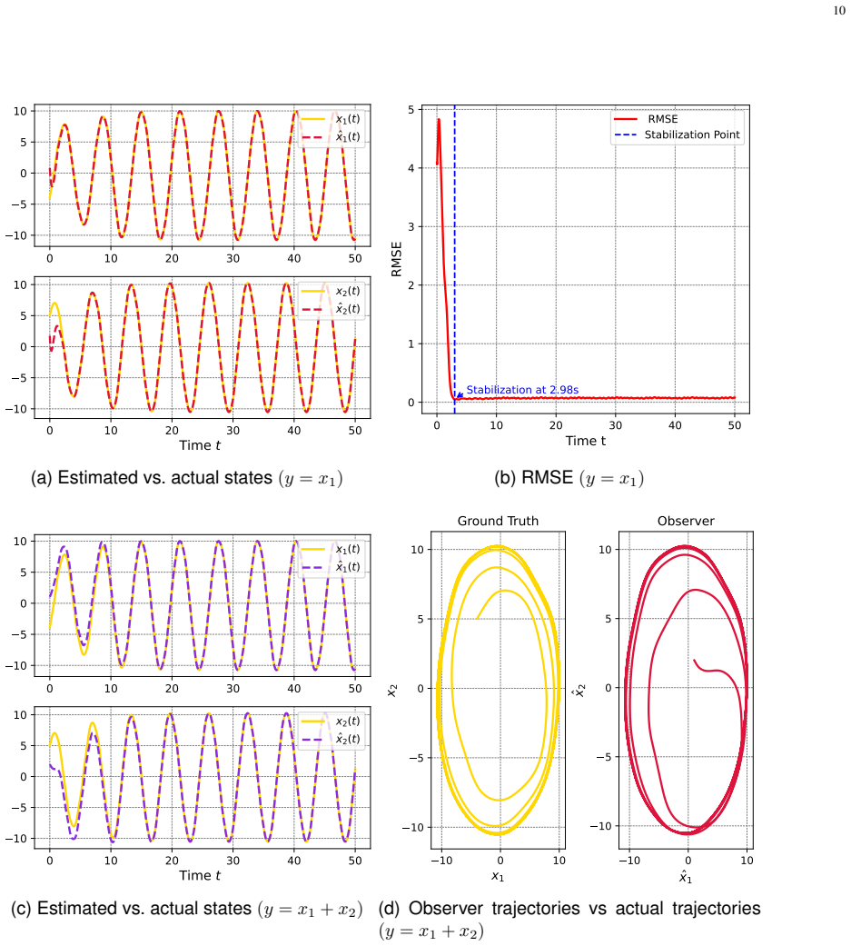
On the reverse Duffing benchmark, the paper reports lower MSE, RMSE, MAE, and SMAPE than supervised neural networks, unsupervised autoencoders, and supervised physics-informed neural networks, with and without noise.

Reading between the lines

Editorial extensions of the paper, not claims the author makes directly.

A reader could settle the practical reach of the theorem by recording $\|L_k-L_k^*\|$ during training on one of the paper’s benchmarks and checking whether it follows an exponential envelope; the paper supplies no architecture or training guarantee that it does.
The same physics-based loss could plausibly be adapted to output-feedback control, where the learned time-varying gain would close the loop as well as correct estimates.
Because the sliding-mode gain depends only on the output error, a natural extension is to asynchronous or fused sensor measurements; the loss already accepts any output map $h$.
The square-wave three-tank experiment suggests a stress test: introducing measurement dropout or sensor bias and observing whether the time-varying gain remains stable would probe the real-time adaptability claim beyond the reported simulations.

Share X Bluesky LinkedIn Reddit HN

Signed reviews

No signed human review yet.

Editorial analysis

A structured set of objections, weighed in public.

Desk editor's note, referee report, and a circularity audit.

Desk Editor's Note

read the letter

Dear colleague,

Quick take: this is a plausible engineering recipe that is overclaimed as a general theory. The paper combines a Luenberger observer with an NN-generated time-varying gain and a tanh sliding-mode term, and trains the NN with a physics-informed loss that uses only measurements, not ground-truth states. That is a useful direction, and the benchmark set (Rössler, three-tank, reverse Duffing, modified outputs) is more varied than most papers in this area. The comparison numbers in Table III are also encouraging if they hold up. Credit where due: the empirical section is honest about challenges like non-differentiable dynamics and weak observability.

The problems are in the theory and the training objective, and they are load-bearing.

First, Theorem 1's proof breaks at Eq. (30): the claim e^T H^T tanh(H e) >= sigma ||H e||^2 is false for large ||H e|| because tanh saturates. You get linear growth, not quadratic. The sector condition needed for SMC stability simply isn't there in the global form used.

Second, Eqs. (20)-(21) invoke Taylor remainders with quadratic bounds, but Assumption 2 only assumes C^1 with bounded Jacobians. On a compact set, C^1 gives a linear remainder, not quadratic, unless second derivatives are bounded. So the Lyapunov difference bound is not established.

Third, and most serious, is the circularity. Theorem 1 assumes ||epsilon_k|| <= epsilon0 e^{-lambda t_k}, i.e., the NN approximation error decays exponentially. Nothing in Assumption 4, the training procedure, or universal approximation supplies this. Universal approximation is static over a compact set; it gives no pointwise-in-time decay along a trajectory. So the theorem's advertised exponential convergence is essentially assumed, not proved. Corollary 1 retreats to ultimate boundedness, which is the honest statement.

Fourth, the training loss (10)-(13) is inconsistent with the observer (3). MSEd = ||\hat x_{k+1} - f(\hat x_k) - B u_k||^2 omits the correction term L_k(y_k-\hat y_k) and the SMC term nu_k. Minimizing it pushes the observer toward open-loop prediction and suppresses the very correction the NN is supposed to learn. That alone undermines the claim that the network learns a stabilizing gain.

The paper also cites related work fairly, so no issue there, but the absence of code/data makes it hard to verify the empirical claims.

Verdict: I would not trust the theorem, and the training loss needs redesign. The idea might be salvageable with a corrected loss and a Lyapunov analysis that treats the NN error as a bounded disturbance (giving ultimate boundedness, not exponential convergence). As it stands, this is not a sound paper. If it comes to a journal, I'd send it back for major revision only on the condition that the authors fix the loss and either prove a valid sector condition or drop the exponential claim. For an arXiv-level reading group, it's a useful cautionary example of how learning-based observer papers can overclaim.

Recommendation: do not send to peer review in current form; desk reject is defensible. If the authors revise, it could become a legitimate contribution, but the current version is not there.

Referee Report

5 major / 5 minor

Summary. The paper proposes a discrete-time nonlinear observer whose time-varying gain is produced by a multilayer perceptron trained with a loss that combines a dynamics residual, an output error, and weight regularization, together with an adaptive sliding-mode correction term. Section V states Theorem 1, which claims exponential convergence of the estimation error to a bounded region under Assumptions 1-4 and an exponential bound on the neural network approximation error. The paper reports simulations on seven examples, including chaotic, weakly observable, and non-differentiable systems, and compares the method against learning-based observers.

Significance. If the theoretical claim were sound, the framework would be significant: it offers an observer design that avoids linearization and coordinate transformations and uses only measured outputs for training. The empirical part covers diverse benchmarks and reports favorable error metrics relative to supervised NN, unsupervised AE, and supervised PINN baselines, which is a genuine strength of the paper. However, the central convergence proof is not valid as stated, and the key exponential-error assumption is neither derived from the training procedure nor verified in the experiments; the contribution is therefore currently an empirical observer design without a rigorous stability guarantee.

major comments (5)

[V, Step 8, Eq. (30)] The inequality e^T H^T tanh(H e) >= sigma ||H e||^2 for some global sigma > 0 is false because tanh saturates. For any scalar z, z tanh(z) behaves like |z| as |z| tends to infinity, so z tanh(z) >= sigma z^2 cannot hold for all z with a fixed sigma > 0; the same holds componentwise for the vector expression. Consequently the lower bound on the SMC contribution used in Step 9, condition (32), does not follow, and the Lyapunov decrease attributed to the sliding-mode term is unproven.
[V, Eqs. (20)-(21), Assumption 2] Equations (20)-(21) assert quadratic remainder bounds ||delta_f(e)|| <= M_f/2 ||e||^2 and ||delta_h(e)|| <= M_h/2 ||e||^2. These require f and h to be twice continuously differentiable with bounded second derivatives on a convex set containing the segment between x_k and hat(x)_k. Assumption 2 only states continuous differentiability with bounded Jacobians, and the compact set Omega is never defined; moreover Assumption 3 evaluates F_k at hat(x)_k, which is not the evaluation point supplied by the mean value theorem. The proof is therefore not supported by the stated assumptions, and the reuse of M_f and M_h with different meanings adds further ambiguity.
[V, Theorem 1 and Assumption 4] The exponential decay assumption ||epsilon_k|| <= epsilon0 e^{-lambda t_k} is an additional hypothesis of Theorem 1, not a consequence of Assumption 4 or of the training loss (10)-(13). Universal approximation is a static statement on a compact set; it provides no pointwise-in-time decay guarantee for epsilon_k = L_k - L*_k along a trajectory. Since epsilon_k is exactly the discrepancy between the learned and the ideal stabilizing gain, assuming it decays exponentially is close to assuming the conclusion that the observer error converges. Corollary 1 shows that with only boundedness one gets ultimate boundedness, so the advertised exponential convergence rests entirely on this unverified condition.
[V, Step 9, conditions (32)-(33)] Conditions (32) and (33) contain ||e_k|| on the right-hand side, so they are state-dependent and cannot be verified a priori. In particular, (33) requires gamma to exceed a term proportional to ||e_k||, so large initial errors can violate the condition at the start of the very process whose boundedness the theorem aims to establish; no argument is given that the required inequality holds along the trajectory. This makes the stability proof circular at a load-bearing point.
[V, Step 10, Eqs. (34)-(36)] The comparison principle is misstated. From Delta V <= -rho V_k + theta one obtains V_{k+1} <= (1-rho) V_k + theta, and the solution is (1-rho)^k V_0 plus theta/rho, not e^{-rho k} V_0 plus theta/(1-e^{-rho}) unless one assumes V_{k+1} <= e^{-rho} V_k + theta and 0 < rho < 1. The constant theta is never explicitly bounded, and no uniform bounds on lambda_max(P_k) are given, so inequality (36) does not follow from the preceding steps.

minor comments (5)

[V, Assumption 2] Assumption 2 introduces a compact set Omega that is never defined; it should be X or the convex hull of X.
[VI, Example 1 and Table I] Table I lists y = x1 for Example 1, while the Roessler system in Eq. (38) has y = x2; one of the two is a typo.
[VI, Example 4, Fig. 5] The caption of Fig. 5 refers to 'system (43)', but Example 4 concerns system (41); the three-tank system is (43).
[VI, Example 7, Eq. (44)] The system in Eq. (44) is called a reverse Duffing oscillator, but the displayed equations do not match the Duffing oscillator form; please clarify the model or the label.
[VI, Table III] The evaluation reports single-run error metrics without confidence intervals or multiple-seed statistics; comparisons in Table III should state the variability across training runs.

Circularity Check

0 steps flagged · score 2.0 of 10

No substantial circularity: Theorem 1 is a conditional stability result whose exponential decay hypothesis on the NN gain error is unproved, but the conclusion is not built into the hypothesis by construction.

full rationale

The derivation chain is not circular. The observer error dynamics are obtained in Eq. (19), the gain is decomposed as L_k = L*_k + epsilon_k in Eq. (22), and Theorem 1 assumes the gain error decays exponentially, ||epsilon_k|| <= epsilon0 e^{-lambda t_k}, together with a lower bound on the SMC gain. The proof then shows, via a Lyapunov difference bound, that the state estimation error e_k converges exponentially to a bounded region. This is a standard disturbance-to-state implication: epsilon_k is the error between the learned gain and an idealized stabilizing gain, not the state error itself, so assuming its decay does not by itself assign a value to e_k. The conclusion therefore is not identical to the hypothesis, and no equation reduces the advertised convergence to the input assumption by construction. The genuine weakness is that Assumption 4 only asserts a bounded approximation error and Theorem 1 adds the much stronger exponential decay condition without deriving it from the training loss (10)-(13), from any architecture bound, or from the Universal Approximation Theorem. That is an unverified hypothesis and a correctness gap, not circularity. Similarly, Step 8's inequality e^T H^T tanh(H e) >= sigma ||H e||^2 is false for large ||H e||, but that is a proof defect rather than a circular reduction. The only self-citation, [10] by Boutayeb et al., appears in a background sentence about EKF limitations and is not load-bearing. No uniqueness theorem is imported from the authors' prior work, and no ansatz is smuggled in via self-citation. Therefore the manuscript does not exhibit substantive circularity; the score reflects only the minor, non-load-bearing self-citation.

Assumptions & free parameters 5 free parameters · 8 assumptions · 0 invented entities

The theoretical result is carried almost entirely by assumptions. Assumption 4 and the exponential error decay are ad hoc, and the proof silently adds smoothness and sector conditions that are not in the assumptions. The loss and observer equations are also internally inconsistent (Eq 11 vs Eq 3), so the trained object is not clearly the object analyzed.

free parameters (5)

K0 (SMC base gain) = 5
Hand-chosen base gain in the adaptive gain K_k = K0 + alpha ||s_k||^2, used in all experiments (Section VI, parameter settings).
alpha (SMC gain scaling) = 0.01
Hand-chosen scaling for the adaptive SMC gain; no tuning analysis is provided.
lambda (regularization weight) = 0.001
Weight of the L2 regularization term in the loss (Eq 13), fixed for all examples.
epsilon0, lambda_exp (exponential NN error bound) = unknown
Theorem 1 assumes the NN approximation error satisfies ||epsilon_k|| <= epsilon0 e^{-lambda_exp t_k}; these constants are never estimated or bounded by the training procedure.
NN architecture (two hidden layers, 64 neurons) = 2x64, tanh, Xavier
Hand-chosen hyperparameters; no sensitivity or width/depth analysis is provided.

assumptions (8)

domain assumption Assumption 1: State trajectories remain in a compact set X for all k.
Used throughout the Lyapunov proof to bound f, h, and their Jacobians; stated in Section V.
domain assumption Assumption 2: f and h are continuously differentiable with bounded Jacobians on X.
Section V; needed for the mean value theorem decomposition, though not sufficient for the quadratic remainder bound used later.
domain assumption Assumption 3: Uniform observability of the linearized system, with the observability Gramian bounded as alpha I <= sum (H Phi)^T(H Phi) <= beta I.
Stated in Section V; used to justify the existence of a stabilizing gain L*_k.
ad hoc to paper Assumption 4: An ideal stabilizing gain L*_k exists and the NN approximates it with bounded error.
The existence is asserted, not constructed, and the error bound is freely chosen.
ad hoc to paper Exponential decay of NN approximation error: ||epsilon_k|| <= epsilon0 e^{-lambda t_k}.
Assumed in Theorem 1; no training guarantee or numerical check is provided, and it mirrors the desired convergence.
ad hoc to paper Quadratic Taylor remainder bound: ||delta_f|| <= M_f ||e||^2/2 and similarly for delta_h.
Used in Step 1 of Proof 1 but not justified by Assumption 2; it requires bounded second derivatives that are not assumed.
ad hoc to paper Riccati inequality solvability: existence of L*_k and P_k with A^T P_{k+1} A - P_k <= -gamma P_k.
Step 7 of the proof asserts this follows from a discrete-time Riccati approach without giving a construction or verifying the assumptions.
ad hoc to paper tanh sector inequality: e^T H^T tanh(H e) >= sigma ||H e||^2 for some sigma > 0.
Used in Step 8; this inequality is false globally because tanh saturates, so no positive sigma exists for all e.

how reviews work

0 comments

Cite this review

Pith. "Pith review of Designing Robust Software Sensors for Nonlinear Systems via Neural Networks and Adaptive Sliding Mode Control." pith.science (2026). https://pith.science/paper/T4557L6I

@misc{pith2026250706817,
  author       = {Pith},
  title        = {Pith review of: Designing Robust Software Sensors for Nonlinear Systems via Neural Networks and Adaptive Sliding Mode Control},
  year         = {2026},
  howpublished = {\url{https://pith.science/paper/T4557L6I}},
  note         = {Machine review of arXiv:2507.06817}
}

read the original abstract

Accurate knowledge of the state variables in a dynamical system is critical for effective control, diagnosis, and supervision, especially when direct measurements of all states are infeasible. This paper presents a novel approach to designing software sensors for nonlinear dynamical systems expressed in their most general form. Unlike traditional model-based observers that rely on explicit transformations or linearization, the proposed framework integrates neural networks with adaptive Sliding Mode Control (SMC) to design a robust state observer under a less restrictive set of conditions. The learning process is driven by available sensor measurements, which are used to correct the observer's state estimate. The training methodology leverages the system's governing equations as a physics-based constraint, enabling observer synthesis without access to ground-truth state trajectories. By employing a time-varying gain matrix dynamically adjusted by the neural network, the observer adapts in real-time to system changes, ensuring robustness against noise, external disturbances, and variations in system dynamics. Furthermore, we provide sufficient conditions to guarantee estimation error convergence, establishing a theoretical foundation for the observer's reliability. The methodology's effectiveness is validated through simulations on challenging examples, including systems with non-differentiable dynamics and varying observability conditions. These examples, which are often problematic for conventional techniques, serve to demonstrate the robustness and broad applicability of our approach. The results show rapid convergence and high accuracy, underscoring the method's potential for addressing complex state estimation challenges in real-world applications.

Figures

Figures reproduced from arXiv: 2507.06817 by the authors.

**Figure 2.** Performance of the proposed method on the R [PITH_FULL_IMAGE:figures/full_fig_p008_2.png] view at source ↗

**Figure 3.** Performance of the proposed method on the harmonic oscillator system. (a) Predicted and actual state trajectories for [PITH_FULL_IMAGE:figures/full_fig_p009_3.png] view at source ↗

Figures from the paper (5 more)

**Figure 4.** Figure 4: Performance of the proposed method on the autonomous system (40). (a) Estimated and actual state trajectories over [PITH_FULL_IMAGE:figures/full_fig_p010_4.png]

**Figure 5.** Figure 5: Performance of the proposed method on the academic system (43). (a) State trajectories. (b) Absolute errors over time. [PITH_FULL_IMAGE:figures/full_fig_p011_5.png]

**Figure 6.** Figure 6: Performance of the proposed method on the academic system (42). (a) State trajectories. (b) Absolute errors over time. [PITH_FULL_IMAGE:figures/full_fig_p011_6.png]

**Figure 7.** Figure 7: Three tank system (43). TABLE II: CONTROL EXPERIMENT TASKS FOR THE THREE-TANK SYSTEM. Experiment Control Torque (u1, u2) (1) u1 = u2 = 0 (2) u1 = u2 = ( umax, if sin(5πf t) > 0, umin, otherwise. We conducted two main experiments to evaluate the performance of our mode…

**Figure 8.** Figure 8: Performance of the proposed method on the Three-Tank system. (a) and (b) correspond to Experiment (1), where no [PITH_FULL_IMAGE:figures/full_fig_p013_8.png]

Discussion (0). Continue with ORCID to comment.

Reference graph

Works this paper leans on

32 extracted references · 32 canonical work pages

[1]

Towards gain tuning for numerical kkl observers,

M. Buisson-Fenet, L. Bahr, V . Morgenthaler, and F. Di Meglio, “Towards gain tuning for numerical kkl observers,” IFAC-PapersOnLine, vol. 56, no. 2, pp. 4061–4067, 2023

work page 2023
[2]

Deep learning-based luenberger observer de- sign for discrete-time nonlinear systems,

J. Peralez and M. Nadri, “Deep learning-based luenberger observer de- sign for discrete-time nonlinear systems,” in 2021 60th IEEE Conference on Decision and Control (CDC) . IEEE, 2021, pp. 4370–4375

work page 2021
[3]

Numerical design of luenberger observers for nonlinear systems,

L. d. C. Ramos, F. Di Meglio, V . Morgenthaler, L. F. F. da Silva, and P. Bernard, “Numerical design of luenberger observers for nonlinear systems,” in 2020 59th IEEE Conference on Decision and Control (CDC). IEEE, 2020, pp. 5435–5442

work page 2020
[4]

Learning- based design of luenberger observers for autonomous nonlinear sys- tems,

M. U. B. Niazi, J. Cao, X. Sun, A. Das, and K. H. Johansson, “Learning- based design of luenberger observers for autonomous nonlinear sys- tems,” in 2023 American Control Conference (ACC) . IEEE, 2023, pp. 3048–3055

work page 2023
[5]

Learning robust state observers using neural odes,

K. Miao and K. Gatsis, “Learning robust state observers using neural odes,” in Learning for Dynamics and Control Conference . PMLR, 2023, pp. 208–219

work page 2023
[6]

Nonlinear discrete-time observers with physics-informed neural networks,

H. V . Alvarez, G. Fabiani, N. Kazantzis, I. G. Kevrekidis, and C. Si- ettos, “Nonlinear discrete-time observers with physics-informed neural networks,” Chaos, Solitons & Fractals , vol. 186, p. 115215, 2024

work page 2024
[7]

Remarks about the numerical inversion of injective nonlinear maps,

V . Andrieu and P. Bernard, “Remarks about the numerical inversion of injective nonlinear maps,” in 2021 60th IEEE Conference on Decision and Control (CDC) . IEEE, 2021, pp. 5428–5434

work page 2021
[8]

Observer design for continuous- time dynamical systems,

P. Bernard, V . Andrieu, and D. Astolfi, “Observer design for continuous- time dynamical systems,” Annual Reviews in Control , vol. 53, pp. 224– 248, 2022. 13 0 20 40 60 80 100 120 140 0 2 x1(t) x1(t) 0 20 40 60 80 100 120 140 0 2 x2(t) x2(t) 0 20 40 60 80 100 120 140 Time t 0 2 4 x3(t) x3(t) (a) State trajectories for Experiment (1) (No control) 0 20 40 ...

work page 2022

Show all 32 references

[9]

Robust extended kalman filtering,

G. A. Einicke and L. B. White, “Robust extended kalman filtering,” IEEE transactions on signal processing , vol. 47, no. 9, pp. 2596–2599, 1999

1999
[10]

Convergence analysis of the extended kalman filter used as an observer for nonlinear deter- ministic discrete-time systems,

M. Boutayeb, H. Rafaralahy, and M. Darouach, “Convergence analysis of the extended kalman filter used as an observer for nonlinear deter- ministic discrete-time systems,” IEEE transactions on automatic control, vol. 42, no. 4, pp. 581–586, 1997

1997
[11]

An adaptive sliding-mode observer for a class of uncertain nonlinear systems,

H. R ´ıos, D. Efimov, and W. Perruquetti, “An adaptive sliding-mode observer for a class of uncertain nonlinear systems,” International Journal of Adaptive Control and Signal Processing , vol. 32, no. 3, pp. 511–527, 2018

2018
[12]

Deep-learning based kkl chain observer for discrete-time nonlinear systems with time-varying output delay,

Y . Marani, I. N’Doye, and T. M. Laleg-Kirati, “Deep-learning based kkl chain observer for discrete-time nonlinear systems with time-varying output delay,” Automatica, vol. 171, p. 111955, 2025

2025
[13]

Data-driven estimation using an echo-state neural network equipped with an ensemble kalman filter,

D. Goswami, A. Wolek, and D. A. Paley, “Data-driven estimation using an echo-state neural network equipped with an ensemble kalman filter,” in 2021 American Control Conference (ACC) . IEEE, 2021, pp. 2549– 2554

2021
[14]

On the computational power of circuits of spiking neurons,

W. Maass and H. Markram, “On the computational power of circuits of spiking neurons,” Journal of computer and system sciences , vol. 69, no. 4, pp. 593–616, 2004

2004
[15]

Echo state networks are universal,

L. Grigoryeva and J.-P. Ortega, “Echo state networks are universal,” Neural Networks, vol. 108, pp. 495–508, 2018

2018
[16]

Neural network adaptive observer design for nonlinear systems with partially and completely unknown dynamics subject to variable sampled and delay output mea- surement,

X. Zhuang, Y . Tian, H. Wang, and S. A. Ali, “Neural network adaptive observer design for nonlinear systems with partially and completely unknown dynamics subject to variable sampled and delay output mea- surement,” Neurocomputing, vol. 561, p. 126865, 2023

2023
[17]

Unsuper- vised physics-informed neural network-based nonlinear observer design for autonomous systems using contraction analysis,

Y . Marani, T. Al-Naffouri, T.-M. Laleg-Kirati et al. , “Unsuper- vised physics-informed neural network-based nonlinear observer design for autonomous systems using contraction analysis,” arXiv preprint arXiv:2411.09237, 2024

2024 arXiv
[18]

Hybrid state estimation: integrating physics- informed neural networks with adaptive ukf for dynamic systems,

J. de Curt `o and I. de Zarz`a, “Hybrid state estimation: integrating physics- informed neural networks with adaptive ukf for dynamic systems,” Electronics, vol. 13, no. 11, p. 2208, 2024. 14 TABLE III: COMPARISON OF ERROR METRICS FOR DIFFERENT MODELS WITH AND WITHOUT NOISE. T...

2024
[19]

Fuzzy neural network-based adaptive sliding-mode descriptor observer,

Z. Zhong, H.-K. Lam, M. V . Basin, and X.-J. Zeng, “Fuzzy neural network-based adaptive sliding-mode descriptor observer,” IEEE Trans- actions on Fuzzy Systems , vol. 32, no. 6, pp. 3342–3354, 2024

2024
[20]

Neural network observer based on fuzzy auxiliary sliding-mode-control for nonlinear systems,

M. Taimoor, X. Lu, W. Shabbir, and C. Sheng, “Neural network observer based on fuzzy auxiliary sliding-mode-control for nonlinear systems,” Expert Systems with Applications , vol. 237, p. 121492, 2024

2024
[21]

Neural-based event-triggered observer design for adaptive sliding mode control of nonlinear net- worked control systems,

Y . Yang, S. Fan, X. Meng, and B. Jiang, “Neural-based event-triggered observer design for adaptive sliding mode control of nonlinear net- worked control systems,” International Journal of Systems Science , vol. 56, no. 4, pp. 850–865, 2025

2025
[22]

Design of a deep neural network-based integral sliding mode control for nonlinear systems under fully unknown dynamics,

E. Vacchini, N. Sacchi, G. P. Incremona, and A. Ferrara, “Design of a deep neural network-based integral sliding mode control for nonlinear systems under fully unknown dynamics,” IEEE Control Systems Letters, vol. 7, pp. 1789–1794, 2023

2023
[23]

Convergence of nonlinear observers on Rn with a riemannian metric (part ii),

R. G. Sanfelice and L. Praly, “Convergence of nonlinear observers on Rn with a riemannian metric (part ii),” IEEE Transactions on Automatic Control, vol. 61, no. 10, pp. 2848–2860, 2015

2015
[24]

A new observer for an unknown harmonic oscillator,

L. Praly, A. Isidori, and L. Marconi, “A new observer for an unknown harmonic oscillator,” in Proceedings of the 17th International Sympo- sium on Mathematical Theory of Networks and Systems, Kyoto, Japan , 2006, pp. 24–28

2006
[25]

Convergence of nonlinear observers on Rn with a riemannian metric (part i),

R. G. Sanfelice and L. Praly, “Convergence of nonlinear observers on Rn with a riemannian metric (part i),” IEEE Transactions on Automatic Control, vol. 57, no. 7, pp. 1709–1722, 2011

2011
[26]

Convergence of nonlinear observers on Rn with a riemannian metric (part iii),

——, “Convergence of nonlinear observers on Rn with a riemannian metric (part iii),” IEEE Transactions on Automatic Control , 2023

2023
[27]

Liquid level tracking control of three-tank systems,

S. Yu, X. Lu, Y . Zhou, Y . Feng, T. Qu, and H. Chen, “Liquid level tracking control of three-tank systems,” International Journal of Control, Automation and Systems , vol. 18, no. 10, pp. 2630–2640, 2020

2020
[28]

Predictive control of three-tank-system utilizing both state-space and input-output models,

M. Kubal ˇc´ık and V . Bob ´al, “Predictive control of three-tank-system utilizing both state-space and input-output models,” sign, vol. 2, no. 1, p. 1, 2016

2016
[29]

3-tank system liquid level control using metaheuristic algorithm,

A. Sharma, H. Goud, and M. K. Kar, “3-tank system liquid level control using metaheuristic algorithm,” in 2023 IEEE Renewable Energy and Sustainable E-Mobility Conference (RESEM) . IEEE, 2023, pp. 1–5

2023
[30]

Adaptive fault-tolerant control for a three-tank system with height and rate constraints,

J. Tang, S. Zhao, Q. Fu, Z. Liu, and W. He, “Adaptive fault-tolerant control for a three-tank system with height and rate constraints,” in 2021 China Automation Congress (CAC). IEEE, 2021, pp. 4020–4024

2021
[31]

Observing a three-tank system,

M. Hou, Y . Xiong, and R. J. Patton, “Observing a three-tank system,” IEEE transactions on control systems technology , vol. 13, no. 3, pp. 478–484, 2005

2005
[32]

Three tank system identification based on genetic algorithm,

M. B. H. Ahmed, N. Majdoub, T. Ladhari, and F. M’Sahli, “Three tank system identification based on genetic algorithm,” in 2020 17th International Multi-Conference on Systems, Signals & Devices (SSD) . IEEE, 2020, pp. 979–984

2020

Pith tools

Reviewed August 6, 2026 · model on record in the stance chip above.

[1] [1]

Towards gain tuning for numerical kkl observers,

M. Buisson-Fenet, L. Bahr, V . Morgenthaler, and F. Di Meglio, “Towards gain tuning for numerical kkl observers,” IFAC-PapersOnLine, vol. 56, no. 2, pp. 4061–4067, 2023

work page 2023

[2] [2]

Deep learning-based luenberger observer de- sign for discrete-time nonlinear systems,

J. Peralez and M. Nadri, “Deep learning-based luenberger observer de- sign for discrete-time nonlinear systems,” in 2021 60th IEEE Conference on Decision and Control (CDC) . IEEE, 2021, pp. 4370–4375

work page 2021

[3] [3]

Numerical design of luenberger observers for nonlinear systems,

L. d. C. Ramos, F. Di Meglio, V . Morgenthaler, L. F. F. da Silva, and P. Bernard, “Numerical design of luenberger observers for nonlinear systems,” in 2020 59th IEEE Conference on Decision and Control (CDC). IEEE, 2020, pp. 5435–5442

work page 2020

[4] [4]

Learning- based design of luenberger observers for autonomous nonlinear sys- tems,

M. U. B. Niazi, J. Cao, X. Sun, A. Das, and K. H. Johansson, “Learning- based design of luenberger observers for autonomous nonlinear sys- tems,” in 2023 American Control Conference (ACC) . IEEE, 2023, pp. 3048–3055

work page 2023

[5] [5]

Learning robust state observers using neural odes,

K. Miao and K. Gatsis, “Learning robust state observers using neural odes,” in Learning for Dynamics and Control Conference . PMLR, 2023, pp. 208–219

work page 2023

[6] [6]

Nonlinear discrete-time observers with physics-informed neural networks,

H. V . Alvarez, G. Fabiani, N. Kazantzis, I. G. Kevrekidis, and C. Si- ettos, “Nonlinear discrete-time observers with physics-informed neural networks,” Chaos, Solitons & Fractals , vol. 186, p. 115215, 2024

work page 2024

[7] [7]

Remarks about the numerical inversion of injective nonlinear maps,

V . Andrieu and P. Bernard, “Remarks about the numerical inversion of injective nonlinear maps,” in 2021 60th IEEE Conference on Decision and Control (CDC) . IEEE, 2021, pp. 5428–5434

work page 2021

[8] [8]

Observer design for continuous- time dynamical systems,

P. Bernard, V . Andrieu, and D. Astolfi, “Observer design for continuous- time dynamical systems,” Annual Reviews in Control , vol. 53, pp. 224– 248, 2022. 13 0 20 40 60 80 100 120 140 0 2 x1(t) x1(t) 0 20 40 60 80 100 120 140 0 2 x2(t) x2(t) 0 20 40 60 80 100 120 140 Time t 0 2 4 x3(t) x3(t) (a) State trajectories for Experiment (1) (No control) 0 20 40 ...

work page 2022